


 text new page (beta)
 English (pdf)
 Article in xml format
 Article references
 Send this article by e-mail
 Cited by SciELO
  Similars in
SciELO
Similars in
SciELO 
 Permalink
Introduction
After the collapse of the Bretton Woods system of fixed exchange rates, in early 1973, most of the developed countries floated their exchange rates. Consequently, this generalized floating regime has been responsible for an increasing volatility of exchange rates, which has been a constant source of concern for policymakers and academics, and also provided data for several empirical works found in the literature analyzing the effects of the exchange rate volatility (ER volatility) on trade flows. The exchange rate volatility is defined as the risk associated with unexpected exchange rate movements, that is, exchange rate risk increases transaction costs and reduces the gains from trade.
According to Sauer and Bohara (2002), due to factors such as degree of risk aversion, hedging opportunities, the currency used in contracts, or the presence of other types of business risk, the direction and magnitude between exchange rate uncertainty (risk) and trade is an empirical question that needs to be investigated.
According to Ozturk (2006), Hooper and Kohlhagen (1978), among other authors, the volatility of the exchange rate is a source of risk and has consequences on the volume of international trade and, therefore, on the balance of payments. These theories suggest that the higher the volatility of the exchange rate, the higher the cost for risk-averse traders and, therefore, a smaller foreign trade. This is because the exchange rate was agreed at the time of the commercial contract, but payment is only made when delivery has been made.
However, the main findings in the literature are far from conclusive, since the effect of ER volatility on trade flows can be both negative (Bittencourt, Larson, & Thompson, 2007; Clark, Tamirisa, & Wei, 2004; Cushman, 1988; Dell’Ariccia, 1999; Hooper & Kohlhagen, 1978; Rose, 2000; Thursby & Thursby, 1987) as positive (Hwang & Lee, 2005; McKenzie, 1998; McKenzie & Brooks, 1997), or the result may be insignificant (Aristotelous, 2001; Gagnon, 1993; Kumar & Dhawan, 1991).
Ozturk (2006) highlights that the ambiguity of the results is associated with the choice of the sampling period, specification of the empirical model, proxy for the ER volatility and the countries considered in the study, that is, whether these are developed or developing countries.
On the other hand, if exchange rates become unpredictable, this creates uncertainty in terms of profits, generating a reduction of these in international trade. Even if there were protection in the markets, there are also cost limitations. In addition, other theoretical developments suggest that there are situations in which ER volatility is expected to have both negative and positive effects on the volume of trade. De Grauwe (1988) pointed out that if the impact of the income effect is greater than the substitution effect, this can lead to a positive relationship between trade and ER volatility, which depends on the degree of risk aversion of exporters. Thus, if exporters are sufficiently risk-averse, an increase in ER volatility suggests a higher expected marginal utility of export earnings, and, therefore, induces increased exports.
The majority of studies about ER volatility and trade flows is based on cross-country analysis (Clark et al., 2004; Cushman, 1988; Dell’Ariccia, 1999, Rose, 2000; Silva, Freitas, & Mattos, 2016; Thursby & Thursby, 1987, among others), while a much smaller number of country-specific studies are available (Arize, 1995; Aurangzeb, Stengos, & Mohammad, 2005; Bittencourt & Campos, 2014; Bittencourt & Correa, 2021; Koray & Lastrapes, 1989; Kumar & Dhawan, 1991; Thi Thuy & Thi Thuy, 2019), from which there are only few studies about ER volatility and trade for South American countries, most of them for Argentina, Brazil and Chile, and only one was found for Colombia (Kandilov & Leblebicioglu, 2015).
Therefore, the main goal of this study is to investigate the main impacts of the bilateral ER volatility on Colombian sectoral exports for its main trade partners for the period 2001-2019, with the use of control variables in addition to ER volatility measure, such as countries’ GDP, distance, and dummy variables for contiguity and common language.
Regarding Colombia’s trade dynamics in recent years, Colombia has participated in several trade agreements, among which is (FTA) with the United States (2011), Mexico (1995), with the countries of the Northern Triangle (2009 -2010) with Mercosur (2004-2005), with Canada (2010), among others. Therefore, it is important for Colombian authorities and policymakers to better understand the country’s trade pattern and the main influences to its exports that comes from ER volatility, in order to seek more stable monetary policies and keep increasing gains from trade.
One way to analyze the effects of ER volatility on Colombian exports is through a gravity trade model, which is widely used in many empirical studies. This model is based on the fundamentals of any economy, such as production, distance, bilateral exchange rate, and it also includes dummy variables to capture various phenomena.
We use three different approaches applied to a panel data of Colombian exports to 11 main trade partners and 97 sectors/products: Pooled OLS, Fixed and Random Effects estimators, and Pseudo-Poisson Maximum Likelihood (PPML) approach.
Therefore, this study brings new insights to this already large literature on ER volatility and trade because it is performed to an important South-American economy, Colombia, which was, as far as we know, investigated by only one published study, and it is a plant-level work (Kandilov & Leblebicioglu, 2015). Hence, our study brings innovative empirical procedures, which includes different model specifications, a sectoral/product disaggregation data, includes a set of control variables not usually employed in such estimations, contiguity and common language, and also different time-window measures of ER volatility for robustness checking.
The main estimation results show a very robust negative impact of the ER volatility to Colombian exports in most of the specified models. The importer´s income seems to affect positively the Colombian exports and, as expected, distance reduces exports for all estimations. The contiguity and common language seem to have a mixed role in explanining trade between Colombia and its main partners for the analyzed period. These findings suggest some policy implications in managing the exchange rate system and promoting exports of Colombia.
In addition to this introduction, the article is divided into four sections. In the next section, a brief review of the literature is carried out on the relationship between exchange rate volatility and international trade. The third section presents the empirical strategy adopted in this study. The fourth section reports the analysis and discussion of the results. Finally, the last section has the final considerations.
Literature review
There is an extensive empirical literature trying to verify the existence of a relationship between exchange rate variability and trade. In this section, representative studies are presented in order to identify the main factors that explain the differences between them. Most of the contributions on the subject have used two different specifications: import or export functions, and gravity models with four different econometric techniques: cross-sectional regressions, time series analysis, panel data, and the method Poisson Pseudo Maximum Likelihood (PPML).
Gravity model
The gravity model is considered by many trade experts as a logic model to explain trade relations between countries. The gravity trade model is developed from the theory of the force of attraction between bodies, which is commonly applied in Physics. The first economists to apply the gravity model of international trade were Tinbergen (1962) and Pöyhönen (1963), who organized the basic variables of the gravity equation. According to Tinbergen (1962), the main determining factors for the success of trade are the size of the countries and their geographical distance.
Subsequently, the model has been improved and used in further studies. According to Bergstrand (1989), based on his analysis of supply prices, he determined that the effects could have an additional variable to include in the gravity equation. Effects are called unobservable events that affect the variables completely or partially, the effects that can be fixed or random. In fact, monopoly competition models have allowed for a solid economic foundation lacking in the gravity equation, which over time has been highly empirically successful.
Therefore, this model has shown to adapt more precisely to the reality of prices, in order to explain bilateral trade in a series of equations related to simple models of monopolistic competition, thus proposing the importance of including multilateral price terms for importers and exporters, in order to determine bilateral trade.
Furthermore, in recent years, the gravity equation has had extensive empirical success, as it better fits the reality of the data, in addition to explaining bilateral trade more precisely.
Bergstrand (1989) examined the theory of Linnemann (1966), creating three categories for each of the explanatory variables of trade. The first category shows the total potential supply of the exporting country in the world market, while the second one speaks of the total potential demand of the importing country in the world market and, finally, the third represents the bilateral “resistance” to trade. According to the author, supply and potential demand are determined by the same forces: the sizes of household products, which influence the scale factor adjustment, and population, which marks the relationship between production for the domestic market and the foreign market. However, in terms of resistance factors, Linnemann highlights the natural obstacles, the best known of which are shipping costs. Additionally, there is time, embedded in transport, since it generates uncertainty in the economic horizon and/or psychological distances, which enlarge a lack of knowledge of the market, its institutions, laws, customs, among others. These factors are usually represented by geographic distance.
Among many applications, Rose (2000) estimates the effect of belonging to a monetary union on international trade flows. In this study, the author estimates that bilateral trade tends to be higher in countries that use the same currency, in contrast to a pair of countries that retained their sovereign currency. The results obtained by Rose are in agreement with the results expected by a gravity trade model, that is, the variables are positively related to GDP and negatively to distance.
Anderson and Van Wincoop (2003) suggest the use of a variable, which they called “multilateral resistance” to be added to the original/modified gravity trade model. According to this variable, exports depend not only on bilateral trade costs, but also on relative bilateral trade costs, that is, a measure of the trade costs of both countries relative to all other countries, in addition to the variables already specified in previously developed models. The authors assume the model for the SBTC (Symmetric Bilateral Trade Cost) hypothesis, according to which for the different countries the costs are symmetric and may not be taken into account when solving the model.
Furthermore, Wilson et al. (2003), used trade facilitation indicators to explain trade flows of manufactured goods between 1989 and 2000, divided into four categories: environmental efficiency, customs, environmental regulations and the use of electronic commerce. This type of indicator can be obtained from mainly qualitative information. Therefore, using gravity equations, one can show that the three facilitation measures generate the expected results and the expected sign. Thus, the improvement in the efficiency of the ports, customs issues and the use of electronic commerce can improve the flow of goods and services. However, environmental regulations have a negative, but significant effect, since they are configured as barriers to trade that replace traditional barriers. Summing up, main results suggest that improvements in the efficiency of ports, in the customs environment and the use of electronic commerce can significantly increase trade.
Based on Wilson, Mann, and Otsuki (2003), Helble, Shepherd, and Wilson (2007) also evaluated trade facilitation within the Asean-Pacific Economic Cooperation (APEC) economies. Authors used the principal components technique to construct two indices that summarize a series of facilitation indicators. The relations between trade flows and these indices were calculated using a gravity model. The authors conclude that APEC’S potential trade gain is higher than those estimated by the reduction of the bilateral tariff and no duty barriers.
Shepherd and Wilson (2008), weighted the impact of bilateral trade facilitation of the member countries of the Association of Southeast Asian Nations (ASEAN). The results showed that trade in these countries is influenced by transportation infrastructure and information technology.
Sadikov (2007) uses a standard gravity model with a sample of 140 countries, in which includes the number of documents needed to export and the number of company registration procedures. The main variable used in the model is a proxy for the frontier and the second one evaluates the measures “within the frontier”. The results showed that, for each additional document established for export, there is a reduction of up to 4.2% in exports, with an impact equivalent to a 5% increase in import tariffs.
Meanwhile, Ordóñez (2010) proposes a gravity model supported and adapted to the one proposed by Anderson and Van Wincoop (2003) in order to study the impact of institutional proximity and institutional distance in bilateral trade using the Zero Inflated Poisson method (ZIP). The results of the study suggest that the two nations that enjoy a good institutional structure tend to have a greater trade flow, compared to two nations with different institutional qualities. However, two nations with low institutional quality tend to trade less than two countries with different institutional qualities. Institutional distance appears to be favorable for bilateral trade, taking into account that institutional distance is relatively less costly in exports compared to Foreign Direct Investment (FDI).
In Colombia, Cárdenas and García (2004) analyzed the impact of a possible FTA between Colombia and the United States through the use of a gravity trade model. They concluded that an (FTA) between Colombia and the United States would increase bilateral trade by 40.5%, however, trade would fall by 57.6% if the agreement was not signed. It is important to bear in mind that the results are only based on partial equilibrium, since any increase in multilateral trade has an inevitable impact on Colombia’s GDP. In addition, other estimates were made with data on imports from the United States by economic sector and they found larger effects. It is important to note that the database includes a measure of shipping costs, which allows a more complete analysis of bilateral trade. Finally, Cárdenas and García reached an important conclusion, that transportation costs (measured as the CIF/FOB ratio at the sector level) are determinants of trade, since the elasticity of the United States imports with respect to transportation costs, was -0.5%, so a 10% reduction in these costs would increase a country’s exports to the United States by 5%.
Effects of the exchange rate volatility
The relationship between ER volatility and trade flows is complex, creating different views pertaining this issue. Even though the level of the exchange rate is important for competitiveness of exports, traders are more concerned about the volatility of exchange rate than its level. The literature that analyzes the effects of ER volatility on international trade emerged in the mid-1970s, after the collapse of the Bretton Woods system, and with the adoption of floating exchange rate regimes, the concern to analyze the impact of the volatility of the nominal and real exchange rates on international trade has increased.
Following Hooper and Kohlhagen (1978), a large number of studies has been published trying to unveil the relationship between ER volatility and trade. However, the theoretical and empirical literature is not conclusive on the effects of such an impact, since the evidence indicates positive, negative, neutral results or a combination of the three (Coric & Pugh, 2010; Ozturk, 2006). These differences can be attributed to the methodological differences of the countries analyzed, the specification of the volatility of the exchange rate used, the sample periods and the time series used (Ozturk, 2006), and also to the fact that traders and other economic agents respond differently to uncertainty, which comes from the random movement of the exchange rate. According to the latter, exporters would be incurring the risk of future conversion of revenues as a result of the unpredictability of the exchange rate, where some exporters would reduce the exposure to the risk while others would see this situation as an opportunity to increase profits.
In general, there are studies on ER volatility and trade from different perspectives. Most of them focus on groups of developed countries and aggregated trade, with little concern about different ways to measure ER volatility, but there are fewer studies that focus on individual emerging-market countries, and a more disaggregated sectoral trade.1 Most of the studies that looked at developed countries found that there is a negative relationship between ER volatility and exports. These include, Clark (1973), Cushman (1988), Brada and Mendez (1988), Koray and Lastrapes (1989), Chowdhury (1993), Dell’Ariccia (1999), Aristotelous (2001), among others.
The seminal study of Hooper and Kohlhagen (1978) examined the impact of the ER volatility on aggregated and bilateral trade for G-7 countries (except Italy), and they found no empirical evidence of a negative effect. On the other hand, Cushman (1983), using an extended sample size and a similar model to that of Hooper and Kohlhagen, found a negative and siginificant effect of the ER volatility for six of a total of 14 bilateral trade flows investigated.
Chowdhury (1993) used an error correction model and focused on G-7 countries, using data between 1973-1990. Through the use of a moving average standard deviation as a measure of ER volatility, this study found a negative and significant relationship between ER volatility and exports, stressing the presence of risk-averse exporters in these countries.
Dell’Ariccia (1999) uses a gravity model and panel data to investigate the ratio of the probability of exchange rate behavior and trade with data from 15 Western European countries. The empirical evidence for this work was based on the hypothesis that exchange rate instability is detrimental to international trade. However, according to the results, the negative effect of ER volatility on international trade was significantly small.
Brada and Mendez (1988) analyzed the effects of exchange rate regimes on the exports of developed and developing countries, including 15 Latin American countries, from 1973 to 1977, using a gravity model.2 They found that the ER volatility is negatively related to exports.
Caballero and Corbo (1989) use a Koyck-type model and real bilateral ER volatility measure to estimate an export demand equation for six countries, among them Chile, Colombia, and Peru. They conclude that there is a strong negative effect of real exchange rate uncertainty on the exports of all these countries.
Silva et al. (2016) estimated a gravity model to investigate the impact of the ER volatility on trade flows among the South American countries for the period of 1997-2011. They used a Poisson-Pseudo Maximum Likelihood (PPML) approach, and they found that instability of exchange rate is detrimental to trade among these countries.
When considering studies about a specific country, instead of a group of countries, Coes (1981) uses a log-level specification to examine Brazilian exports for the period 1965-1974 and concludes that a significant reduction in ER volatility in the country’s economy during the crawling-peg era had a positive effect on the country’s exports after the crawling peg was adopted in 1968.
Mustafa and Nishat (2004) investigated the relationsip between ER volatility and export growth considering Pakistan’s earliest trading partners for the period 1991-2004. The results suggest negative effects of the empirical relationship between export growth and ER volatility with respect to Australia, New Zealand, the United Kingdom and the United States. However, for Bangladesh and Malaysia no evidence was found in this regard. Subsequently, Mukhtar and Malik (2010) took the study of Mustafa and Nishat (2004) as a point of reference, looking again at the case of Pakistan, but at this time the authors considered global exports and a GARCH specification to evaluate the ER volatility for the period 1960-2007. The authors found no statistical evidence of such relationship.
Bittencourt et al. (2007) studies the effects of the volatility of the real exchange rate on Brazilian sectoral trade in Mercosur during the period 1989-2002. The authors used gravity trade equations, where the dependent variables represent the volume of bilateral trade of five sectors (Agriculture, Animal Production, Chemicals, Manufacture and Mining), while the explanatory variables represented two measures of the ER volatility, import tariffs, the GDP of the countries, the geographical distance, and a measure for the “third country” volatility that represents the effect of the ER volatility of a third trading partner, under the bilateral trade considered. Among the results, it was observed that the exports from four of the total five sectors analyzed (Agriculture, Chemicals, Manufacture, Mining) were negatively affected by the volatility of the exchange rate.
Bittencourt and Campos (2014) investigates the impact of currency instability on the export and import flows of Brazil with its main trading partners between 1989 and 2011. Estimates based on the gravity model revealed that trade flows between Brazil and its trading partners were negatively affected by the ER volatility for all the sectors analyzed.
Vargas Torres (2014) empirically investigates the impact of the ER volatility on Colombian trade with its major trading partners under the flexible exchange rate regime for the period 2000-2012. Long-run estimates of cointegration analysis were obtained using Johansen’s approach and estimates of short-term dynamics were obtained using a vector error correction (VEC) model. The results showed that increases in the ER volatility cause reduction in the Colombian exports.
Kandilov and Leblebicioglu (2015) is the only published study3 found so far that investigates the relationship between ER volatility and trade in Colombia. However, this study uses a plant-level panel data and uses a system-GMM estimator. Using two different ER volatility measures, GARCH model and a simple standard deviation measure, they found a small negative impact of ER volatility on trade. They conclude that the negative impact of ER volatility is stronger for small or moderate size plants, since they are more likely to enter international markets when they experience small export incentives.
Another different perspective when analyzing the relationship between ER volatility and trade, is about the methodology, where many studies use the error correction models, including Coes (1981), Thursby and Thursby (1987), Cushman (1988), De Grauwe (1988), Arize (1990) and Dell’Ariccia (1999). However, there are studies that use different approaches. Koray and Lastrapes (1989), for instance, apply a Vector Autoregressive (var) model to bilateral trade between Germany, Canada, France, United Kingdom and United States. They found a weak relationship between ER volatility and trade in the short-run, which, if sustained, could cause risk aversion and a negative impact on exports in the long-run. Some other studies use panel data econometrics, such as Cho, Sheldon, and McCorriston (2002), Bittencourt et. al (2007), Carmo and Bittencourt (2014), Silva et al. (2016), among others.
McKenzie (1999) is a very comprehensive survey of empirical studies about ER volatility and trade. His survey of the empirical studies brings the same mixed picture of results, with many studies finding no significant effect or, where significant, no systematic effect in one direction or the other. However, the most recent contributions to the literature have been more successful in showing a statistically significant relationship between ER volatility and trade, which he believes that is due to more careful attention to the specification of the estimation technique and the measure of volatility used.
Concluding this review, a set of meta-analyses can be useful to represent an extensive literature regarding the effects of the ER volatility on international trade, such as the studies of Ozturk (2006) and Coric e Pugh (2010). These studies confirm the majority of findings of negative effects of exchange rate volatility on international trade.4
Methodology and data
Data
In order to identify the effect of ER volatility on Colombian trade with its main trading partners, a panel data model is estimated using data for 11 countries (Brazil, Chile, China, Ecuador, Mexico, Netherlands, Panama, Peru, Spain, United States, Venezuela) for the years between 2001 and 2019. The data were taken from various sources. Colombian exports were obtained from Trade Map (International Trade Centre), with information provided by the United Nations. The export values were taken with a two-digit level of disaggregation, generating a sample of 97 products.
The values of the real exchange rate for all 11 countries were taken from World Development Indicators, and these values are expressed in terms of the US dollar. Regarding the countries’ GDP data, they were provided by the World Bank, and their values are expressed in millions of dollars for the period 2001-2019. The data about the distance between Colombia and its trade partners are from Centre D’Estudes Prospectives at d’Informations Internationales (CEPII).
Dependent variable
The dependent variable to be used is the Colombian exports (exp ijt ), exports from country i (Colombia) to country j (trade partners) at each year t.
The Colombian main destination countries represent, on average, 70% of exports for the period 2004-2019. Table 1 shows the annual exports’ share for each of the 11 Colombian trade partners since 2004.
Table 1 Colombian exports for its main destination countries (%)
| BRA | CHL | CHI | ECU | MEX | NLD | PAN | PER | SPA | USA | VEN | Total | |
|---|---|---|---|---|---|---|---|---|---|---|---|---|
| 2004 | 0.8 | 1.5 | 0.8 | 6.0 | 3.1 | 2.3 | 1.2 | 3.2 | 1.3 | 42.0 | 9.7 | 72.0 |
| 2005 | 0.9 | 1.4 | 1.1 | 6.2 | 2.9 | 2.1 | 1.2 | 3.3 | 1.6 | 41.7 | 9.9 | 72.5 |
| 2006 | 0.8 | 1.0 | 1.8 | 5.0 | 2.4 | 2.1 | 1.0 | 2.8 | 2.1 | 41.0 | 11.0 | 71.1 |
| 2007 | 1.6 | 1.2 | 2.6 | 4.2 | 1.6 | 2.8 | 0.8 | 2.7 | 1.9 | 35.4 | 17.4 | 72.4 |
| 2008 | 1.7 | 2.3 | 1.2 | 4.0 | 1.6 | 2.0 | 0.8 | 2.3 | 1.7 | 38.0 | 16.2 | 71.8 |
| 2009 | 1.8 | 2.9 | 2.9 | 3.8 | 1.6 | 4.1 | 0.9 | 2.4 | 1.5 | 40.0 | 12.3 | 74.2 |
| 2010 | 2.6 | 2.3 | 4.9 | 4.6 | 1.6 | 4.0 | 2.3 | 2.8 | 1.4 | 43.0 | 3.6 | 73.2 |
| 2011 | 2.4 | 3.9 | 3.5 | 3.3 | 1.2 | 4.4 | 3.4 | 2.4 | 3.0 | 38.5 | 3.1 | 69.3 |
| 2012 | 2.1 | 3.6 | 5.5 | 3.2 | 1.4 | 4.1 | 4.8 | 2.6 | 4.9 | 37.0 | 4.2 | 73.6 |
| 2013 | 2.7 | 2.7 | 8.7 | 3.4 | 1.5 | 3.9 | 5.5 | 2.2 | 4.9 | 32.0 | 3.8 | 71.2 |
| 2014 | 3.0 | 1.8 | 10.5 | 3.4 | 1.7 | 3.9 | 6.6 | 2.2 | 6.0 | 26.4 | 3.6 | 69.1 |
| 2015 | 3.3 | 2.1 | 6.3 | 4.0 | 2.6 | 4.2 | 6.7 | 3.2 | 4.4 | 28.2 | 3.0 | 68.1 |
| 2016 | 3.2 | 2.2 | 3.6 | 3.9 | 3.0 | 3.9 | 6.2 | 3.4 | 3.7 | 33.0 | 2.0 | 68.1 |
| 2017 | 3.6 | 2.7 | 5.3 | 3.9 | 4.1 | 4.1 | 6.8 | 3.0 | 2.6 | 29.2 | 0.8 | 66.2 |
| 2018 | 3.7 | 2.8 | 9.7 | 4.4 | 3.9 | 2.5 | 7.3 | 2.8 | 2.8 | 27.1 | 0.8 | 68.1 |
| 2019 | 3.7 | 2.4 | 11.5 | 4.9 | 3.6 | 3.1 | 5.9 | 2.9 | 1.3 | 31.0 | 0.5 | 70.9 |
| Mean | 2.4 | 2.3 | 5.0 | 4.3 | 2.4 | 3.3 | 3.9 | 2.8 | 2.8 | 35.2 | 6.4 | 70.7 |
Note: BRA (Brazil), CHL (Chile), CHI (China), ECU (Ecuador), MEX (Mexico), NLD (Netherlands), PAN (Panama), PER (Peru), SPA (Spain), USA (United States), VEN (Venezuela).
Source: Elaborated by the authors based on data from Trade Map (International Trade Centre).
According to Table 1, the United States is the main destination country for the Colombian exports, being responsible, on average, for almost 35% of total exports. In recent years, China became the second main destination for Colombian exports. It is interesting to note the changes in theses figures for some countries over time. For instance, considering Venezuela’s share on Colombian exports, we can see how much these numbers decreased since 2009, when Venezuela’s share was 12.3%, and declined substantially since then, reaching, approximately, 0.5% in 2019. On the other hand, Brazil’s share shows a totally opposite behavior, with only 0.8% of the Colombian exports in 2004, but achieving 3.7% in 2019.
Overall, it seems like China, the Netherlands, Panama and Spain were the destinations for Colombian exports that “replaced” the Venezuela purchases of Colombian products since 2009, since the export shares for these countries increased substantially since then.
Figure 1 shows the structure of product exports from Colombia to the rest of the world in 2006 and 2019. The product category with the largest share in 2019 corresponds to the sector of mineral fuels, oils and waxes, with a 54% share, followed by the coffee/tea sector with a share of 6%. We can see that these figures slightly change when compared to 2006 for some of the sectors. The main variation was in the sector of mineral fuels, oils and waxes, which increased its share in almost 50% in the period considered. However, the sectors of vehicles other than railway, iron and steel, and sugars experienced a large drop in the participation on total Colombian exports from 2006 to 2019.
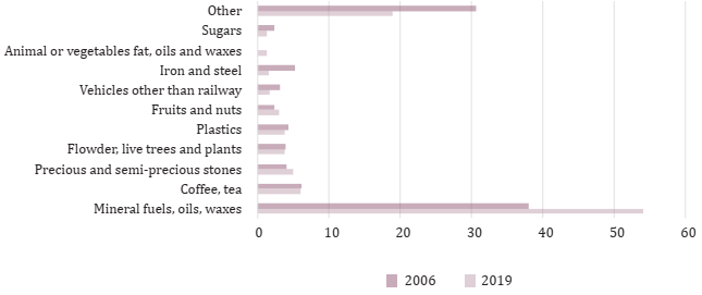
Source: Elaborated by the authors based on UN Comtrade Database.
Figure 1 The structure of product exports for Colombia in 2006 and 2019 (% share on total exports)
The comparison showed in Figure 1 also emphasizes a substantial increase in the concentration of the Colombian exports, since these products were responsible for 70% of total exports in 2006, but this number went up to 81% in 2019.
Independent variables
The gravity model to be estimated will include, as independent variables, countries’ GDP, distance, a measure of ER volatility, and dummy variables for contiguity and common language. Therefore, GDP it represents the gross income of Colombia at time t, and GDP jt the gross income of each trade partner at time t. According to Bittencourt (2004), as this variable represents a proxy for income, it is reasonable to assume that the higher the income level of the countries, the greater the quantity of products demanded. Additionaly, it is implicit that the higher the income of a country, the greater the diversity of products that are demanded. Likewise, this variable is expected to have a positive effect on Colombian exports.
On the other hand, DIST ij is the geographical distance from Colombia (country i) and the trading partners (country j). This variable is an indicator of transport costs (Nilsson, 1999). Therefore, it is reasonable to assume that geographic distance is a natural barrier to trade. This coefficient is expected to have a negative effect on Colombian trade flows.
LANG ij is a dummy variable that assumes a value equal to 1 when both countries speak Spanish, and 0 otherwise. According to Andersson (2007), sharing the same language can mitigate communication costs between countries and improve trade between them, as seen in Piani and Kume (2000).
FRONTij is a dummy variable that assumes a value 1 when the country j has common border with Colombia (country i), and 0 otherwise. It is believed that when countries have common borders, transportation costs are reduced by increasing trade flows between countries, as seen in Jordán and Parré (2006). So, the coefficient associated with this variable is expected to have a positive sign in the estimated model.
VOLijt represents the measure of bilateral ER volatility of Colombia and each of its main partners. In order to estimate the relationship between the bilateral ER volatility on trade between Colombia and its main trading partners, a volatility measure is used based on the studies of Frankel and Wei (1993), Dell’Ariccia (1999), Rose (2000), Bittencourt et al. (2007) and Tenreyro (2007). According to these authors, there is no consensus about the best way to measure the bilateral volatility of the exchange rate, therefore, this work relies on the usual moving standard deviation, described as:
Where Xij,t is the real bilateral
exchange rate, xij,t =
ln(Xij,t) -
ln (Xij,t-1),
and k = 2, 3, and 4 years.5
According to many authors, such as Frankel and Wei (1993), Dell’Ariccia (1999), Rose (2000), Bittencourt et al. (2007), Tenreyro (2007), Carmo and Bittencourt (2014), the use of a measure of ER volatility using lags larger than one can avoid endogeneity problems in the model, and this is the reason for using different values for k in equation (1).
Figure 2 depicts the calculated ER volatility given by the moving standard deviation for the previous four years for only few countries of the sample: Brazil, Chile, China and Colombia. The behavior of the ER volatility for the remaining countries of the sample are not so different than those represented in Figure 2. The exceptions are Venezuela, the Netherlands and Spain. The ER volatility for Venezuela is high in the last years of the sample, and the opposite occurs for the two European countries.
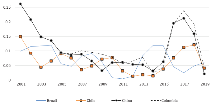
Source: Elaborated by the authors based on data from World Bank.
Figure 2 The ER volatility calculated using the moving standard deviation (k = 4) for selected countries, for the period 2001-2019
There is a similar behavior of the ER volatility between China and Colombia. Large volatility is apparent in both countries in the first and in the last years of the sample. Brazil’s ER volatility seems to have a different pattern when compared to the others. There is an overall decline in the ER volatility in most of the four countries considered in the Figure 2.
The empirical model
In this work we use an extended gravity model accounting for the volatility of bilateral real exchange rate in order to analyze the behavior of Colombian exports with its main trading partners with respect to exchange rate fluctuations for the period from 2001 to 2019. The econometric specification of the gravity model plays a fundamental role in the proper estimation of the marginal effects of each independent variable on trade. Therefore, the gravity model to be estimated is given by:
In order to analyze the effect of ER volatility on trade between Colombia and its main partners, the gravity equation to be specified is a modified version of the basic equation. In addition, the econometric approaches to estimate the model take different forms, including the Pooled OLS model, panel data estimations by random and fixed effects models, and the Poisson Pseudo Maximum Likelihood method (PPML).
Since equation (2) has as its dependent variable the natural logarithm of Colombian exports, this can create a problem, since the database used in this study has 97 products/sectors for 19 years, and it is likely to have a considerable number of zeros in the sample, with no exports of such products to some trading partners. Therefore, the PPML technique was chosen to estimate the gravity equation and avoid the zero-trade-flows problem. According to Santos Silva and Tenreyro (2006), additional advantages on adopting the PPML approach are: unbiased estimates in the presence of heteroscedasticity, since it is robust to different patterns of heterocedasticity; all observations are equally weighted, since the variance is assumed proportional to the mean; and the mean is always positive. This estimation is based on the replacement of the dependent variable lnEXPijt by EXPijt in equation (2).
According to our data, the dependent variable EXPijt has a zero value for 4 561 observations, which will be excluded from the estimates using the direct specification given by equation (2).
Results and discussion
Firstly, we present the main descriptive statistics for the variables of the gravity model. It follows with the main empirical results from all econometric approaches: Pooled OLS, fixed effects estimations, random effects estimations and PPML. Finally, we have a sub-section that summarizes the main findings about the influence of the ER volatility on Colombian exports.
According to Table 2, there are 4 561 observations with no trade flows in the sample. The Colombian GDP (GDPit) has a lower mean than the GDP of its main trade partners, but it is larger than some of its trade partners, such as Ecuador, Panama, Peru and Venezuela. The ER volatility has different features depending on the number of years (k) used for its calculation. For instance, larger values used for k imply in a higher mean for the ER volatility. As expected, Spanish is the main language spoken in 64% of the countries considered in the sample: Chile, Ecuador, Mexico, Panama, Peru, Spain and Venezuela; and Colombia has borders with 45% of its main trade partners: Brazil, Ecuador, Panama, Peru and Venezuela.
Table 2 Main descriptive statistics for the variables of the gravity model
| Variable | Obs. | Mean | Standard deviation | Min | Max |
|---|---|---|---|---|---|
| lnEXPijt | 15 712 | 6.700 | 2.992 | 0 | 16.593 |
| lnGDPit | 20 273 | 26.131 | 0.481 | 25.273 | 26.668 |
| lnGDPjt | 20 273 | 27.020 | 1.852 | 23.249 | 30.695 |
| lnDISTij | 20 273 | 8.033 | 0.989 | 6.496 | 9.611 |
| VOLijt (k = 2) | 20 273 | 0.099 | 0.365 | 0.00001 | 5.018 |
| VOLijt (k = 3) | 20 273 | 0.139 | 0.412 | 0.002 | 4.839 |
| VOLijt (k = 4) | 20 273 | 0.187 | 0.485 | 0.004 | 4.709 |
| LANGij | 20 273 | 0.636 | 0.481 | 0 | 1 |
| FRONTij | 20 273 | 0.454 | 0.497 | 0 | 1 |
Source: Author’s calculations.
All models were estimated using different window lags for the ER volatility measure (k = 2, 3, 4). The results showed that there were no significant changes between the estimated models. Therefore, in most of this section we will present the estimates from ER volatility based on the 4-year lag measure. The estimates obtained by the regression model Pooled, Fixed Effects, Random Effects and Poisson Pseudo Maximum Likelihood (PPML) are presented, respectively. All tables represent different model specifications. In addition to the variables in the first column, the following columns have the estimate results taking into account year-fixed effects, product/sector-fixed effects, or both fixed effects. In the last columns we have the full version of the gravity model, including all the variables expressed in equation (2), that is, including common language and border variables, followed by year-fixed effects, product/ sector-fixed effects, and both.
Pooled OLS estimations
According to the results from the Pooled OLS estimations, given by Table 3, all the coefficients were statistically significant and with the expected signs. The only exceptions were the ones associated to the Colombian GDP, which was not significant in the specifications 1 and 5, but this coefficient was significant and negative for all other estimations. The results also suggest that if the additional income of Colombian trading partners varies, the additional income resulting from this variation will be used to purchase more Colombian products. According to the first column of Table 3, an increase of 1% in the GDP of the trading partners generates an increase of 0.48% in the volume of exports of Colombian products by the trading partner market.
Table 3 Estimation results from the Pooled OLS model
| Pooled OLS | ||||||||
|---|---|---|---|---|---|---|---|---|
| lnEXPijt | 1 | 2 | 3 | 4 | 5 | 6 | 7 | 8 |
| lnGDPit | -0.041 | -0.316** | -0.111* | -0.408* | -0.080 | -0.384* | -0.171* | -0.514* |
| (0.05) | (0.12) | (0.04) | (0.09) | (0.06) | (0.12) | (0.04) | (0.09) | |
| lnGDPjt | 0.481* | 0.484* | 0.605* | 0.609* | 0.511* | 0.515* | 0.653* | 0.659* |
| (0.02) | (0.02) | (0.01) | (0.01) | (0.02) | (0.02) | (0.02) | (0.02) | |
| lnDISTij | -1.278* | -1.285* | -1.715* | -1.725* | -1.451* | -1.461* | -1.976* | -1.991* |
| (0.04) | (0.04) | (0.03) | (0.03) | (0.05) | (0.05) | (0.04) | (0.04) | |
| lnVOLitj | -0.266* | -0.288* | -0.305* | -0.336* | -0.292* | -0.321* | -0.344* | -0.385* |
| (0.03) | (0.03) | (0.02) | (0.02) | (0.03) | (0.03) | (0.02) | (0.02) | |
| CONST | 4.318* | 11.309* | 2.939* | 12.248* | 5.861* | 13.607* | 5.231* | 15.723* |
| (1.36) | (3.15) | (1.03) | (2.33) | (1.42) | (3.16) | (1.06) | (2.29) | |
| LANGij | - | - | - | - | 0.304* | 0.308* | 0.472* | 0.477* |
| - | - | - | - | (0.08) | (0.08) | (0.06) | (0.06) | |
| FRONTij | - | - | - | - | -0.505* | -0.508* | -0.753* | -0.760* |
| - | - | - | - | (0.09) | (0.09) | (0.06) | (0.06) | |
| Year FE | - | Yes | - | Yes | - | Yes | - | Yes |
| Product FE | - | - | Yes | Yes | - | - | Yes | Yes |
| OBS. | 15 712 | 15 712 | 15 712 | 15 712 | 15 712 | 15 712 | 15 712 | 15 712 |
| R2 | 0.080 | 0.081 | 0.551 | 0.552 | 0.086 | 0.086 | 0.562 | 0.564 |
Note: Standard errors in parenthesis; *** p<0.10, ** p<0.05, * p<0.01.
Source: Author’s calculations.
For all specifications, the estimated coefficients for distance were negative and significant. The estimated coefficients for distance were between -1.3 and -2.0. Since distance generates a factor that hinders trade, the greater the distance between trading partners, the higher the transportation costs, and the prices of the traded products increase in the same way. If transportation costs increase by 1%, the distance between Colombia and its trading partners causes a -1.3% drop in the volume of exports, considering the estimated coefficient for distance in the first column. Dennis and Shepherd (2007) and Bittencourt et al. (2007) also found that geographical distance has a negative impact on the patterns of geographical diversification of exports.
The estimated coefficients for ER volatility varied between -0.26 and -0.38 for all specifications in Table 3. Therefore, an increase of 1% in the ER volatility would reduce the Colombian exports, approximately, in 0.3-0.4%.
As expected, the estimated coefficients for common language and border (frontier) dummies were all significant (columns 5-8, Table 3). It is interesting to note that the estimates for common language were positive, while the estimates for border were negative, which can indicate that speaking Spanish can increase Colombian exports, while trading with neighboring countries can reduce exports.
These results make sense, mainly considering that the trade flows in 2019 from Colombia to all Spanish-speaker countries in the sample (Chile, Ecuador, Mexico, Panama, Peru, Spain, Venezuela) corresponds to 22% of total Colombian exports, while this proportion of total Colombian exports corresponds only to 18% for neighboring countries (Brazil, Ecuador, Panama, Peru, Venezuela). However, the negative coefficients for the border dummies are not surprising, since Colombian exports for no-neighboring countries (Chile, China, Mexico, the Netherlands, Spain, United States) were around 53% in 2019, mainly with the United States and China.
Figure 3 represents the scatterplot and the linear adjustment between actual and predicted log of Colombian exports. It can be seen that the small export values are repeated more often throughout the sample. For instance, there are 4 products/sectors (observations) with the same export value of us$ 271 000: cocoa products for Chile in 2001, wood products for Ecuador in 2007, fish and other aquatic invertebrates for Mexico in 2012, and vehicles and parts other than railway for Spain in 2017. If we consider us$ 1 000 export value, there are 372 observations in the sample, and they become 372 zeros after taking the natural logarithm of exports, which can be seen as the first column of points in Figure 3.

Panel data estimations
According to Table 4, we have the results from the fixed and random effects models. The estimated coefficients for Colombian GDP were positive and significant for most of the specifications (except for specifications 4, 6 and 8), which is expected by the theory, but it is the opposite than it was obtained from the Pooled OLS results. The estimated coefficients for the Colombian trade partners’ GDP were once again positive and significant for all specifications, varying between 0.2 and 0.4. These estimates were lower in magnitude than the ones from the Pooled OLS.
Table 4 Estimation results from the panel data model
| Fixed Effects | Random Effects | |||||||
|---|---|---|---|---|---|---|---|---|
| lnEXPijt | 1 | 2 | 3 | 4 | 5 | 6 | 7 | 8 |
| lnGDPit | 0.342* | 0.171*** | 0.264* | 0.063 | 0.182* | 0.090 | 0.198* | -0.026 |
| (0.08) | (0.10) | (0.07) | (0.10) | (0.06) | (0.11) | (0.06) | (0.09) | |
| lnGDPjt | 0.217** | 0.198** | 0.305* | 0.303* | 0.397* | 0.276* | 0.377* | 0.381* |
| (0.09) | (0.10) | (0.07) | (0.07) | (0.05) | (0.08) | (0.06) | (0.06) | |
| lnDISTIj | - | - | -1.203* | -1.205* | -1.458* | -1.784* | -1.962* | -1.977* |
| - | - | (0.12) | (0.13) | (0.09) | (0.20) | (0.12) | (0.12) | |
| lnVOLItj | -0.248* | -0.297* | -0.251* | -0.296* | -0.255* | -0.298* | -0.257* | -0.302* |
| (0.03) | (0.03) | (0.03) | (0.03) | (0.03) | (0.03) | (0.03) | (0.03) | |
| CONST | -8.653* | -3.883** | -0.141 | 4.969** | 0.743 | 10.422* | 5.514* | 11.179* |
| (1.46) | (1.89) | (1.54) | (2.19) | (1.45) | (2.79) | (1.89) | (2.34) | |
| LANGij | - | - | - | - | - | -0.307 | -0.045 | -0.049 |
| - | - | - | - | - | (0.31) | (0.20) | (0.21) | |
| FRONTij | - | - | - | - | - | -1.283* | -1.260* | -1.271* |
| (0.36) | (0.21) | (0.21) | ||||||
| Year FE | - | Yes | - | Yes | - | Yes | - | Yes |
| Product FE | - | - | - | - | Yes | - | Yes | Yes |
| OBS. | 15 712 | 15 712 | 15 712 | 15 712 | 15 712 | 15 712 | 15 712 | 15 712 |
| R2 | 0.090 | 0.097 | 0.090 | 0.098 | 0.089 | 0.098 | 0.090 | 0.097 |
Note: Standard errors in parenthesis; *** p<0.10, ** p<0.05, * p<0.01.
Source: Author’s calculations.
Since there are no estimates for time-invariant variables in a fixed-effects model, we need to rely only on a random-effects model to get such estimates. Therefore, the estimated coefficients for distance, from specifications 3-8, were all negative and significant, showing similar magnitude to the same estimations from the Pooled OLS.
Frontier and common language dummies are additional time-invariant variables in the gravity model, which random effects estimates showed negative and significant coefficients for Frontier (border), and no significant estimates for common language. According to Table 4, Colombian trade with a neighboring country can reduce exports in a larger proportion than observed from the Pooled OLS estimates, which is not a surprise since a considerable proportion of the Colombian exports are with the United States and China, as mentioned before. However, we have distinct results when we look at the estimated coefficients for common language dummies. While these estimates were positive and significant in Table 3, the estimates from random-effects models are not significant, that is, on average, the Colombian exports do not change because its partner is a Spanish-speaker country.
Table 4 shows that the estimated coefficients for ER volatility were all negative and statistically significant, which means that, on average, the greater the instability of the bilateral real exchange rate, the lower the Colombian exports will be. In other words, an increase in exchange rate volatility increases trade costs between Colombia and its trading partners, which has a negative impact on total trade between them. Following Rose (2000), both instability and currency fluctuations are associated with greater risk and uncertainty on the part of economic agents, which can represent a disincentive that harms international trade activities. The results shown in all specifications indicate that ER volatility has a negative effect on trade dynamics, as a 1% increase in ER volatility could cause a reduction of, approximately, 0.3% in the volume of Colombian exports, considering the second column of Table 4. The negative effect of ER volatility in trade between countries derives from the theory of choice of uncertainty. This theory emphasizes that, in situations of uncertainty, economic agents choose the option that offers the least risk, if they are risk averse. The application of these assumptions to trade means that, in situations in which the volatility of the exchange rate makes activity related to the external market uncertain, the producer agents choose activities in which the risk is lower. That is, choose activities for the domestic market (Cho et al., 2002).
PPML estimations
The most appropriate approach we used was the Poisson Pseudo Maximum Likelihood (PPML) method (Table 5), since its results are consistent in the presence of heteroscedasticity and considers all 20 273 observations, including the zero-values in the sample. Based on the results obtained through the different specifications, it is observed that almost all of the estimated coefficients for lnGDPit and lnGDPjt were positive and statistically significant. These results corroborate the findings from the literature. The results are also in agreement with the central hypothesis of the gravity model, with a positive relationship between income and trade. The estimates varied between 0.5 and 0.8 for the Colombian GDP, and 0.4 to 0.7 for the trading partner’s GDP. It is believed that the increase in the level of income of the trading partner occurs in parallel with an increase in the demand for imported products. These results are similar to those found in the studies by Santos Silva and Tenreyro (2006), Helble et al. (2007).
Table 5 Estimation results from the PPML model
| Poisson Pseudo Maximum Likelihood (PPML) | ||||||||
|---|---|---|---|---|---|---|---|---|
| EXPijt | 1 | 2 | 3 | 4 | 5 | 6 | 7 | 8 |
| lnGDPit | 0.459* | 0.630 | 0.459*** | 0.630*** | 0.682* | 0.808** | 0.682* | 0.808* |
| (0.19) | (0.36) | (0.10) | (0.15) | (0.20) | (0.36) | (0.09) | (0.13) | |
| lnGDPjt | 0.694*** | 0.699*** | 0.694*** | 0.699*** | 0.361* | 0.379* | 0.361* | 0.379* |
| (0.06) | (0.06) | (0.03) | (0.03) | (0.06) | (0.06) | (0.04) | (0.04) | |
| lnDISTij | -0.942*** | -0.935*** | -0.942*** | -0.935*** | -1.381* | -1.366* | -1.381* | -1.366* |
| (0.12) | (0.12) | (0.08) | (0.08) | (0.19) | (0.19) | (0.11) | (0.12) | |
| lnVOLitj | -0.152* | -0.117* | -0.152*** | -0.117** | -0.153** | -0.135** | -0.153* | -0.135* |
| (0.06) | (0.06) | (0.05) | (0.06) | (0.07) | (0.06) | (0.04) | (0.05) | |
| CONST | -14.079** | -18.521 | -18.028*** | -22.470*** | -6.059 | -9.871 | -10.008* | -13.819* |
| (5.27) | (9.53) | (2.66) | (3.87) | (5.18) | (9.54) | (2.71) | (3.91) | |
| LANGij | - | - | - | - | -1.122* | -1.068* | -1.122* | -1.068* |
| - | (0.27) | (0.26) | (0.19) | (0.18) | ||||
| FRONTij | - | - | - | - | -1.290* | -1.248* | -1.290* | -1.248* |
| (0.24) | (0.24) | (0.16) | (0.16) | |||||
| Year FE | - | Yes | - | Yes | - | Yes | - | Yes |
| Product FE | - | - | Yes | Yes | - | - | Yes | Yes |
| OBS. | 20 273 | 20 273 | 20 273 | 20 273 | 20 273 | 20 273 | 20 273 | 20 273 |
Note: Standard errors in parenthesis; *** p<0.10, ** p<0.05, * p<0.01.
Source: Author’s calculations.
As mentioned in the literature review, the variable distance is used in this study as a substitute for transport costs in trade. According to Table 5, it is observed that Colombian exports are inversely related with the distance between the countries considered. This result indicates that if the transportation cost increases by 1%, the volume of trade will decrease by 0.94%, according to estimates in the first column of Table 5. This result is supported by Santos Silva and Tenreyro (2006), which also found smaller coefficients for distance using a PPML model than when using Pooled OLS, and Bittencourt et al. (2007), which analyzed the impact of ER volatility on Mercosur trade, where the authors found similar results for the variable that represents the distance between countries.
The dummy variables for frontier and common language produced negative and significant estimated coefficents. The estimated coefficients for common language (LANGij) showed similar magnitudes to the estimated coefficients for frontier (FRONTij). Therefore, when considering the whole sample, including 4 561 zeroes, the presence of a neighboring country or a Spanish-speaker country as a trade partner actually reduces the overall Colombian exports, considering all other variables constant.
Directing the analysis to the variable that represents the main focus of this study, all the estimated coefficients of ER volatility were negative and statistically significant, which shows that, on average, the greater the instability of the bilateral exchange rate, the lower the total trade between the countries analyzed. That is, on average, an increase of 10% in the ER volatility would reduce exports in 0.12-0.17 thousands of us dollars. These are very small estimates, which are similar to the ones estimated by Koray and Lastrapes (1989), Lastrapes and Koray (1990), Frankel and Wei (1993) and Eichengreen and Irwin (1998), Hondroyiannis, Swamy, Tavlas, and Ulan (2008).
ER volatility and trade
Turning to the main focus of this paper, all model estimations discussed, based on Tables 3, 4 and 5, suggest that the impact of ER volatility is negative and significant considering a moving standard deviation measure using equation (1) with k = 4, that is, using a 4-year lag. However, if we try to get more robustness in our investigation of the impact of ER volatility on Colombian exports, it is necessary to consider other lag windows (k values) for the moving standard deviation measure for ER volatility. Table 6 shows a summary of the estimated coefficient for ER volatility with lag windows of k = 2 and k = 3, for all respective specifications reported in previous tables for k = 4.
Table 6 Summary of the ER volatility estimations
| ER Volatility | Pooled OLS | |||||||
|---|---|---|---|---|---|---|---|---|
| 1 | 2 | 3 | 4 | 5 | 6 | 7 | 8 | |
| k = 2 | -0.072* | -0.097* | -0.098* | -0.133* | -0.077* | -0.103* | -0.106* | -0.143* |
| k = 3 | -0.218* | -0.248* | -0.262* | -0.299* | -0.243* | -0.278* | -0.299* | -0.345* |
| k = 4 | -0.265* | -0.288* | -0.305* | -0.336* | -0.292* | -0.321* | -0.344* | -0.385* |
| Year FE | - | Yes | - | Yes | - | Yes | - | Yes |
| Product FE | - | - | Yes | Yes | - | - | Yes | Yes |
| ER Volatility | Fixed effects | Random effects | ||||||
| 1 | 2 | 3 | 4 | 5 | 6 | 7 | 8 | |
| k = 2 | -0.078* | -0.106* | -0.076* | -0.103* | -0.075* | -0.104* | -0.076* | -0.103* |
| k = 3 | -0.220* | -0.273* | -0.219* | -0.269* | -0.221* | -0.271* | -0.223* | -0.272* |
| k = 4 | -0.248* | -0.297* | -0.251* | -0.296* | -0.255* | -0.298* | -0.257* | -0.302* |
| Year FE | - | Yes | - | Yes | - | Yes | - | Yes |
| Product FE | - | - | - | - | Yes | - | Yes | Yes |
| ER Volatility | PPML | |||||||
| 1 | 2 | 3 | 4 | 5 | 6 | 7 | 8 | |
| k = 2 | -0.028 | -0.060 | -0.028 | -0.060** | -0.019 | -0.049 | -0.019 | -0.049*** |
| k = 3 | -0.123** | -0.105*** | -0.123* | -0.105** | -0.123*** | -0.120** | -0.123* | -0.120* |
| k = 4 | -0.152* | -0.117* | -0.152*** | -0.117** | -0.153** | -0.135** | -0.153* | -0.135* |
| Year FE | - | Yes | - | Yes | - | Yes | - | Yes |
| Product FE | - | - | Yes | Yes | - | - | Yes | Yes |
Note: *** p<0.10, ** p<0.05, * p<0.01.
Source: Author’s calculation.
Comparing all estimated coefficients in Table 6, we can see that most of the estimates are statistically significant, and also that the long-run ER volatility (k = 4) coefficients are larger than the medium (k = 3) or short-run (k = 2) estimates. De Vita and Abbott (2004) also find stronger impacts of ER volatility on exports using a long term volatility based on the past five years (k = 5).
According to Perée and Steinherr (1989), exporters can, relatively easily, insure against short term risk through forward market transactions. However, it is much more difficult and costly to hedge against long term risk. De Grauwe and De Bellefroid (1986) and De Grauwe (1988) argue also that short-run variability is irrelevant to trade, which corroborates the results reported in Table 6 with low coefficients estimated using a short-run measure of volatility with k =2.
Having provided evidence supporting the influence of ER volatility on Colombian exports, we can make a few observations regarding the obtained estimates. Firstly, results reveal a higher long term impact of the real exchange rate, both in terms of significance and magnitude in all models. This would suggest that past information is particularly relevant in order to assess the impact of exchange rate volatility on trade. This analysis confirms much of the existing literature in that short-run effects of the exchange rate on trade are limited. It is, therefore, advisable to concentrate future analysis on longer term effects of exchange rate levels on trade. Secondly, the impact of exchange rate changes on exports found here is echoed in much of the literature (Baek & Koo, 2009; Bahmani-Oskooe & Ardalani, 2006; Haynes, Hutchison, & Mikesell, 1986). Finally, the negative impact of ER volatility on trade found in our estimations confirm the findings from Vargas Torres (2014) and Kandilov and Leblebicioglu (2015) for Colombia, Caballero and Corbo (1989) for Chile, Colombia and Peru, Bittencourt and Correa (2021) for Brazil, Bittencourt et al. (2007) for the Mercosur countries, Silva et al (2016) for South America, among others.
Final considerations
The main objective of this study was to analyze how exchange rate volatility affects the Colombian exports with its main trading partners, between 2001 and 2019. This study contributes to the literature of ER volatility and trade, mainly because it was applied to Colombian trade flows for the first time considering a sectoral data disaggregation and the econometric techniques used, and also for using different time-specifications (lags) for the ER volatility measures.
Even though the literature that relates international trade to changes in the exchange rate is extensive, there is no exact conclusion as to how these volatile effects can affect trade. A large empirical literature finds a negative, positive and mixed relationship between ER volatility and trade. Therefore, in this study, when analyzing such relationships, the results obtained show that ER volatility is detrimental to the commercial relationship between Colombia and its main trading partners, that is, that export performance will be negatively impacted by ER volatility in the long-run. A one percent increase in ER volatility would reduce export volume significantly by about 0.25 to 0.4 percent.
According to Clark et al. (2004), our findings occur because exporting companies are capable of altering production factors in the short term. Thus, companies become more vulnerable to changes in international prices, declining profits, and facing greater difficulty adjusting to exchange rate fluctuations. Therefore, following Baldwin and Krugman (1989), the effects of ER volatility may be different for each sector of the economy as a consequence of the specific characteristics of each sector. The authors argue that sectors with a high initial demand for investment are less affected by ER volatility.
Our gravity model performs well empirically, yielding precise and generally reasonable estimates. The coefficient on distance was negative and statistically significant for all estimated models, and very similar to results from Santos Silva and Tenreyro (2006), Tenreyro (2007), Bittencourt et al. (2007).
As in many other studies, one of the main drivers of trade flows is found to be income -which is specified as domestic income in the case of imports and foreign income in the case of bilateral exports. The coefficients on GDP were positive and statistically significant for most of the estimated models. A rise in national income leads to an increase in the value of domestic imports through the increased purchasing power of Colombian consumers. In a same way, foreign income plays a significant role in determining Colombian exports.
The coefficients for contiguity (border/frontier) and common language, which were included as country-specific control variables, seem to negatively affect Colombian exports, which would be an unexpected result, however, due to the large part of Colombian products be shipped to the United States and China makes this result not so unusual.
Our results have several policy implications. First, and foremost, economic policies that aim to stabilize the exchange rate are likely to increase the volume of trade for Colombia and its trade partners. Second, although considering exchange rate policy, it is essential for the government to adapt synchronous implementation solutions to overcome possible presence of bottlenecks in Colombian exports.
This study can be extended in several directions. First, one could also assess how ER volatility affects Colombian imports and compare with our results for exports. Additionaly, one could also explore different levels of trade disaggregation to see if there are differences in the impacts of ER volatility on sectoral trade. Finally, our work could also be extended by the use of different econometric approaches and measures for ER volatility.

