


 nova página do texto(beta)
 Inglês (pdf)
 Artigo em XML
 Referências do artigo
 Enviar este artigo por email
 Citado por SciELO
  Similares em
SciELO
Similares em
SciELO 
 Permalink
Introduction
When analyzing the effects of shocks, disturbances, or stochastic components that affect an economic system, as an example of a textbook, the most typical cases used are wars and natural disasters because they highlight the imbalances and havoc that they generate on nations. These peculiar shocks are hardly contemplated in the forecasters’ projections, either by the authorities themselves or by the private capital. Now we can add a new issue: Pandemics.
A global economic slowdown already preceded the beginning of 2020 and a growing diplomatic and commercial tension between the countries with the most significant financial (and political) power; however, no one expected a pandemic. The Coronavirus’s emergence in late 2019 in Wuhan, China, was officially declared as pandemic on March 11, 2020, by the World Health Organization (WHO), creating an economic, health, and social damage worldwide.
Studies on epidemics are widely documented in biology, mathematics, and chemistry; however, COVID-19 is a disease that has tried to find answers in other areas of science. In economics, the modeling of a pandemic and its repercussions on the growth and development of countries has been strongly led by the Susceptible Infected Recovered (SIR) epidemiological model dating from 1927 and vehement retaken by economists.
Beyond applying the SIR model in its raw form for economies, we use it to find both the size and the trajectory or dynamics that the pandemic’s tracks (through numerical integration and phase diagrams). We analyze advanced countries and developed countries using the International Monetary Fund (IMF) classification. Subsequently, we use forecasting models derived from machine learning: Ensemble methods.
There is also a limitation in this research since the countries do not have a similar population for direct comparison, or the number of tests carried out to detect Coronavirus, essential variables in our work. However, we want to highlight that the results of each country reveal that, overall, the pandemic can be much larger than the reported statistics. The trajectory that the COVID-19 follows is cyclical and depends on health measures and self-care that this cycle takes less time to reach its lowest point.
The virus’s outbreak is unavoidable, hence the relevance of having a vaccine (such as the H1N1 vaccine that is applied every year in Mexico). Finally, we estimated a low and gradual recovery, but making it clear that one year (2021) is not going to be enough to reach the average growth levels that countries had. Even the growth is not directly incorporated in the SIR model; we add a macro data analysis to present an accurate context of COVID-19 and growth relationship, obtaining results for both long-term Coronavirus dynamics and growth forecasts to 2021.
The structure of the document begins with a brief review of the SIR model literature and its implementation for economic analysis. Subsequently, we present relevant data about infections, deaths, the COVID-19 test, and its correlation with the slump in economic growth. The third part focuses on the methodological tooling implementation, which revolves around the SIR model and is complemented by our predictions. The main findings and conclusions are shown in the last section.
We want to make evident our concern about how the scope of this pandemic may be underestimated. From people who have decided to take care of themselves and those who want to do it, but their conditions do not allow it (whatever the cause). Also, for those fearless and nonbelievers of this disease, we hope to provide a better understanding of the COVID-19 dynamics.
Brief literature review on epidemiological modeling
Before COVID-19, there are just a few papers in the literature that begin to point out the consequences of epidemics in macroeconomic variables, primarily when the avian flu arose (or H5N1 influenza) in 2007, H1N1 influenza in 2009, and the outbreak of Ebola in 2014.
For example, in the work of the European commission written by authors Lars and Werner (2006), they analyze the effects of economic contraction derived from avian flu for the United States and Europe. Pandemic studies are also focused on measuring the loss of crops and their impact on meat demand (Paarlberg, Seitzinger, & Lee, 2007). Likewise, the costs of acquiring vaccines as a proportion of Gross Domestic Product (GDP) have also been analyzed using general equilibrium into Smith, Keogh-Brown, Barnett, & Tait (2009) to verify the amount of GDP of vaccinating children in the United Kingdom against H1N1 influenza.
However, studies on the effects of pandemics on economies remained limited until the arrival of COVID-19, although different documents can be found on the Coronavirus’s ravages in nations and projections on the economic contraction at the national level. Worldwide, research on its size and duration based on their particular conditions of each country is limited. Before continuing with our research proposal, we want to emphasize some articles that have served as the basis for forming this article.
COVID-19 has received attention to the use of the SIR model, since it allows to represent, in a simplified way, the process of virus’s spreading in a population over time. This model was developed by Kermack and McKendrick (1927) and consists of three non-linear ordinary differential equations where the population can only belong to one of the states:
Susceptible: Individuals who are exposed to the virus.
Infected: Individuals who contract the virus.
Recovered or removed: These are the individuals who passed the previous phases and are now recovered.
This model is widely used to study the dynamics of measles and smallpox (Rodrigues, 2016). However, SIR became the reference to perform several analyzes of COVID-19 in 2020. Since the applications of the basic model found in Atkeson (2020) and which is later reproducible in Sargent and Stachurski (2020), to modified versions where public policy evaluations are made on different segments of the population to verify the efficiency of health measures in Acemoglu, Chernozhukov, Werning and Whinston (2020). Likewise, SIR is used to analyze consumers’ decision-making and preferences in the United States and the effects of mobility on absenteeism (Eichenbaum, Rebelo, & Trabandt, 2020).
Besides, the SIR model has also been implemented in Gros, Valenti, Schneider, Valenti and Gros (2020) to analyze the social costs of distancing through a modified SIR that reacts to each change or implementation of new sanitary measures. However, a work more similar to ours is the one carried out by Stock (2020), where different levels of flattening are determined for different levels of contagion so that the efficiency of the confinement measures is also exhibited. Likewise, Toda (2020) shows the heterogeneity in the rate of transmission and spread of the Coronavirus in different countries.
Our study starts with the model in its primary expression. Following numerical integration and phase diagrams, we estimate the pandemic’s size and duration to compute forecasting with different machine learning on the selected advanced economies and emerging market and developing economies. In the next section, we specify the analysis and results obtained.
Macro data and COVID-19 shocks
The COVID-19 pandemic not only has caused millions of deaths but also has impacted on global economy, and Mexico is not the exception. The data of COVID-19 presented in this article was obtained from Our World in Data COVID-19 of Roser, Ritchie, Ortiz-Ospina and Hasell (2020), which gathers daily statistics from various the most countries.
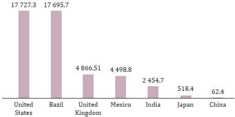
The number of total cases per million inhabitants of the major economies1 is shown in Figure 1.
Source: Authors’ elaboration with data of Our World in Data.
Figure 1 Total cases per million inhabitants as of March 28, 2020
Nowadays, the United States and Brazil are the countries with the highest number of Coronavirus cases in the major economies with 17 727 and 17 695 cases per million inhabitants, respectively. According to the data, between the United States and the United Kingdom total cases, there is a difference of more than double the cases; the United Kingdom has 4 866 cases, which represent 27.4% of the total cases in the United States. On the other hand, Mexico ranks fourth with a total of 4 497.8 cases that depict 8.7 times the number of cases in Japan that are worrisome due to Japan and Mexico have a similar population. Ultimately, China is the country with fewest cases on the list despite being the country where the pandemic began.
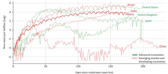
Furthermore, the countries on the list appear to have flattened the curve but not bent it. Figure 2 shows the logarithm of the contagion curve for the major economies; they are classified in advanced economies and emerging market and developing economies.
Source: Authors’ elaboration with data of Our World in Data.
Figure 2 Daily new confirmed cases per million inhabitants as of March 28, 2020
Adjusted per million inhabitants, Mexico has one of the highest daily new confirmed cases only beneath Brazil, United States, and India. Nevertheless, Mexico’s curve is the most stable compared to the rest of the emerging markets and developing economies.
In contrast, as of March 28, 2020, COVID-19 has reached a total of 832 019 confirmed deaths in the world according to official data. The reader should take into account that the actual total number of deaths is likely to be greater than the number of confirmed deaths due to limited evidence and problems in attributing the cause of death, as well as how deaths from COVID-19 may differ between countries, for instance, some countries can only count deaths in hospitals, while others have started to include deaths in homes (Roser et al., 2020).
Focusing only on the major economies, the United Kingdom has the highest number of adjusted deaths per million of inhabitants while China is the economy with the lowest number of deaths, in Table 1 can be appreciated the total confirmed deaths adjusted per million inhabitants, per capita gross domestic product (GDP per capita) obtained from Organisation for Economic Cooperation and Development (OECD, 2020).
Table 1 Total confirmed deaths per million inhabitants as of March 28, 2020
| Country | Deaths per million inhabitants | GDP Per capita 2019 (US Dollars) |
|---|---|---|
| United Kingdom | 610.98 | 48 745 |
| Brazil | 558.19 | 14 592 |
| United States | 546.29 | 65 143 |
| Mexico | 485.48 | 20 703 |
| India | 44.59 | 5 902 |
| Japan | 9.79 | 43 279 |
| China | 3.28 | 14 306 |
Source: Authors’ elaboration with data of Our World in Data and OECD.
In this sense, the United Kingdom, Brazil, the United States, and Mexico have significantly more deaths than India, Japan, and China. Comparing with GDP per capita of the countries, the United Kingdom has 62.4 times more deaths than Japan, Mexico148.2 times more than China, and Brazil has 12.5 times more than India.
Testing is perhaps the most important topic because all the available data comes from it; this means that the counts of confirmed cases, deaths, and spread of the pandemic depend on the number of tests carried out by each country; in this sense, it becomes a fundamental issue for the public and economic policy against the pandemic. Table 2 shows the number of tests per thousand inhabitants, the percentage of these positive tests, and the total adjusted cases per million inhabitants, as well as the daily tests per thousand people.
Table 2 Testing for COVID-19 last available data as of March 28, 2020
| Country | Total cases per million inhabitants |
Total tests per thousand inhabitants |
Positive rate (%) | Daily tests per thousand people |
|---|---|---|---|---|
| United States | 17 727.3 | 246.11 | 5.8 | 2.24 |
| Brazil | 17 695.7 | 22.57 | NaN | 0.43 |
| United Kingdom | 4 866.5 | 183.35 | 0.7 | 2.39 |
| Mexico | 4 497.8 | 9.34 | 52.4 | 0.08 |
| India | 2 454.7 | 28.61 | 7.9 | 1.72 |
| Japan | 518.4 | 13.51 | 4.9 | 1.24 |
| China | 62.4 | NaN | NaN | NaN |
Source: Authors’ elaboration with data of Our World in Data and OECD.
Sorting by total tests, the United States is the country tests more in comparison with the rest of countries with a positive rate of 5.8%; this is a concerning issue for Mexico given that is not only the country with the lowest number tests but also the country with the highest positive rate, and even the most downward daily tests. In the same ratio, the United Kingdom has become in the country with the highest number of daily tests of the major economies.
Economic activity has been seriously affected by the decrease in consumer spending and growth on the unemployment rate, and the partial closure of the so-called non-essential activities has led to forecasts toward lower levels than the financial crisis of 2008. In Figure 3 is shown the forecast of the major economic groups according to the IMF.
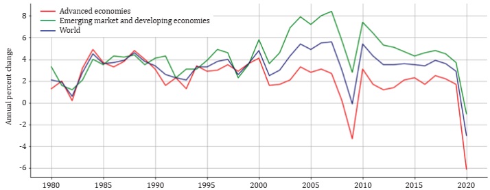
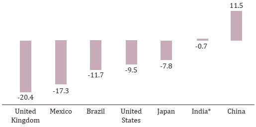
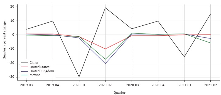
The IMF estimates that economic growth in advanced economies slows by 6.1%. Its forecast for emerging and developing economies has dropped 1%, resulting in a forecast for a 3% global economic recession. Figure 4 shows the economic crunch for the major economies in the second quarter of 2020.
* Growth rate of 01-2020.
Source: Authors’ elaboration with data of OECD.
Figure 4 Quarterly GDP growth, previous period, Q2 2020
The United Kingdom is the country with the deepest economic downturn, followed by Mexico; in contrast, the country where the pandemic began presented an economic recovery of 11.5% compared to the previous quarter; in this sense, China is the only one of the major economies that did not show a drop in the second quarter of 2020.
On the other hand, the leading stock market indices that are represented by the most representative corporations of each stock market and on several occasions reflect the expectations of a country’s economy are showing in Figure 5.
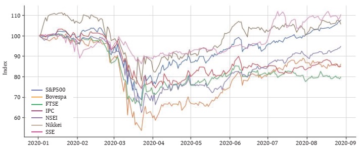
Source: Authors’ elaboration with data of Yahoo Finance.
Figure 5 Stock market performance in 2020 Index 01-02-2020 = 100
As the reader can appreciate, only three of the major stock indices have performed better this year: Standard and Poor’s 5002 (S&P 500), Shangai Stock Exchange Composite (SSE), and Nikkei 225 (Nikkei) from the United States, China, and Japan, respectively. On the other hand, we find that the English index (FTSE) is the one that has performed the worst so far this year, followed by Mexico (IPC) and Brazil (Bovespa) in addition to showing a lateral trend in recent months. India (NSEI), meanwhile, has not yet reached the levels of the beginning of the year. Nevertheless, the trend suggests that it will fully recover in the coming months.
The next section makes a comparison of the size of the pandemic in the countries. Likewise, we make a forecast for the coming quarters, considering the effect of the Coronavirus on economic activity.
Pandemic’s dynamics, phase diagrams, and equilibria
The SIR model works under the assumption that the population is homogeneous, and they have similar characteristics. Each individual can only belong to one state at a time (susceptible, infected, or removed). Also, the three states are time-dependent variables.
As time goes by, the number of susceptible people (St) decreases since they got infected (It). The number of people who go to the new state is weighted by the contagion rate (β); in parallel, people who go from infected to removed or recovered are weighted by the recovery rate (γ). As the pandemic spread, the number of susceptible people can only decrease while the number of infected people increases until the maximum number is reached; likewise, the number of people who recover shows an upward trend. The SIR model is developed using a system of ordinary differential equations, as shown below:
Where:
St = Susceptible population.
It = Infected population.
Rt = Recovered population.
N = Total population.
β = Transmission rate.
γ= Recovery rate.
The model assumes that both β and γ>0.
The γ parameter that represents the recovery rate is nothing more than the inverse of the number of days that a person lasts being infectious (or sick) while the beta parameter represents the transmission rate from the new cases of transmission registered. This β parameter is obtained from a first-order autoregressive (AR1) taking the logarithm of the new cases registered in each country. Different estimation methods are used to find the most suitable contagion rate and are presented in Table 3.
Table 3 Transmission rate β and AR1 results
| Country | Best specification | Infection rate (β) |
|---|---|---|
| United States | Elastic Net | 0.9693 |
| Japan | Elastic Net | 0.9139 |
| United Kingdom | Elastic Net | 0.9592 |
| China | Elastic Net | 0.9160 |
| India | Elastic Net | 0.9566 |
| Brazil | Elastic Net | 0.9518 |
| Mexico | Huber | 0.9473 |
According to the IMF classification, Brazil, India, Mexico, and China belong to the category of emerging and developing economies. In contrast, the United States, Japan, and the United Kingdom have their place to the classification of advanced economies. The inputs to feed the SIR model: Total cases, new cases, new deaths, total deaths, and life expectancy, were taken from the Our World in Data COVID-19 that has the daily pandemic record for the countries considered.
For population size, we used Worldometer data as of July 2020, and an average of 2
weeks for recovery according to the who estimations. In that sense, the recovery
rate is defined as
Where μ refers to life expectancy, for this first approach, it is considered that μ = 0, this means a closed epidemic. When the reproductive rate R0 = 1, the change of the epidemic in the system is observed. Figure 6 exhibits the SIR model with the reproductive rate R0.

SIR model represents N as the whole population of each nation; the time is measured in weeks, so it is possible to realize the peak of the curve; for example, United States, United Kingdom, Brazil, India, and Mexico seem to reach the peak after ten weeks while Japan takes about 18weeks and China more than 20 weeks. Note that the dotted line shows the recovery point. This is where the number of people suspected of being infected begins to decrease. It should be noted that this curve (St) does not converge to 0 since there is always a proportion of the population that is exposed to infection (close to 30% for most countries once the critical stage of transmission passes). Ultimately, no more than 15% of the population becomes infected, making sense since it would represent millions of people infected with the virus.
Regarding the size of the pandemic, we look for equilibrium (if it exists) in the
differential equations proposed for each country. In the case of a closed epidemic,
that is, without considering life expectancy (there are no new births or deaths),
the trajectories of the equations can be integrated through numerical integration.
The susceptible population is defined as 1-f through the implicit
solution
That integrates the curve
If S(0)= N then N-(∞) are the final size of the pandemic, and the infected fraction is:
And integrating numerically, we obtain:
The final sizes for a closed epidemic are presented in Table 4. This is the size that the COVID-19 could reach if there would be no government intervention or sanitary measures.
Table 4 Size of closed epidemics for the countries
| Country | Final size (%) | R0 rate |
|---|---|---|
| United States | 77.92 | 1.9386 |
| Japan | 74.26 | 1.8278 |
| United Kingdom | 77.30 | 1.9131 |
| China | 74.42 | 1.832 |
| India | 77.14 | 1.9132 |
| Brazil | 76.83 | 1.9036 |
| Mexico | 76.55 | 1.8946 |
We add μ parameter to introduce population demographics; this means that the model now becomes endemic (or open) as long as the reproduction rate R0 > 1 . The specification is as follows:
Let E*(S*, I*, R*) the endemic equilibrium of the model, then S *, I *, R * satisfy the equations:
Where N *= S * +I * +R *. Likewise, recall that equilibrium exists when R0 >1 . Therefore, state relations have a unique equilibrium in the following equations. This demonstration can be verified in (Ma, Zhou, & Cao, 2013).
Finally, the phase diagrams are presented in Figure 7. The phase diagrams present spiral trajectories; in other words, the system’s trajectory exhibits cyclical behavior. Arrows pointing inward to the node or equivalence point denotes stability. The United States, India, and China show larger oscillations than the other countries. This does not mean that the cycle necessarily becomes more extended, but instead shows the relationship between susceptible and infected individuals. Mexico, Brazil, United Kingdom, and Japan present more cyclical trajectories but with similar scope to the other countries.

Using the Jacobian matrix for the SIR model:
The Jacobian of the SIR model is:
Which represents the endemic equilibrium for each country. The key to the eigenvalues
is the sign of the root. Negative signs in the diagonal represent global stability,
while positive signs are the opposite and show global instability. The combination
of positive and negative sings refers to a saddle point. The trajectories exhibit
imaginary roots in the diagonal, triggering a spiral path that seams never ends (and
matches with the endemic behavior). The spiral path or internal track is determined
by
Table 5 Length of the pandemic (endemic)
| Country | Length in weeks | Length in years |
|---|---|---|
| United States | 455 | 8.72 |
| Japan | 472 | 9.05 |
| United Kingdom | 456 | 8.74 |
| China | 471 | 9.03 |
| India | 457 | 8.76 |
| Brazil | 459 | 8.80 |
| Mexico | 460 | 8.82 |
The results show that the pandemic can take between 8 and 7 years to finish. The model can also be interpreted as the time it would take for a highly dangerous outbreak to emerge by presenting cyclical behavior. Hence the importance of making public policy decisions. The next section is destined to ensemble model estimations for economic forecasting.
SIR model and ensemble models estimations
Ensemble methods are a machine learning technique that consists of a combination of multiple models to produce the optimal base estimator. This type of algorithm is called ensemble because it improves generalization/robustness in a single estimator (Pedregosa et al., 2011). We decided to use these types of models because they are excellent for non-linear modeling systems of equations; they do not need particular assumptions about data distribution, and they also handle collinearity efficiently. According to (Hastie, Tibshirani, & Friedman, 2009) ensemble methods can characterize any dictionary method, such as regression splines, as an ensemble method. The essential functions of playing weak predictors’ roles ensemble methods are more robust and accurate than parametric models.
For purposes of this article, we forecast with two kinds of ensemble methods: Random Forest regressor and Gradient Boosting regression tree. Random forest was developed by Breiman, (2001), is a collection of three predictors h(x;θk), k = 1, …, K where x represent the observed input vector of length p with an associate random vector X and θk is an independent and identically distributed random vectors.
When Random Forest is used for regression, the predictor is an unweighted average over the collection as follows:
Where k → ∞ by the Law of Large Number ensures.
In general, this method is based on bagging or bootstrap aggregation; each model is trained on the bootstrap sample of the training data enforcing diversity of each tree via random feature selection. The reinforcement improves the forecasting accuracy through variance reduction by averaging many noisy but unbiased trees.
In this sense, trees are ideal candidates for bagging because they can capture complex interaction structures in the data, and if they grow deep enough, they have a relatively low bias; as trees are notoriously noisy, they benefit significantly from the average. Furthermore, as each tree generated in bagging is distributed identically (i.d.), an average B such tree’s expectation is the same as the expectation of any of them. This means that the bagged trees’ bias is the same as that of the individual trees, and the only hope of improvement is through the reduction of variance. This contrasts with improvement, where trees grow adaptively to eliminate bias, and therefore are not i.d. (Hastie et al., 2009); in this sense, the noise is a clear advantage over parametric models due to Random forest fit a better performance with noise, while the parametric model fits better without outliers. Given this, we considered this part of the cycle we are, representing a clear outlier in the long-term growth rate and this kind of model’s decision.
In this way and retaking variables from equation 10, an average of K i.d random variables but not independent and with positive pairwise correlation ρ, the variance of the average is:
As K increases, the second argument of the equation disappears, remaining the variance pondered by correlation. The main idea is to improve the model’s variance by reducing the correlation between the trees and achieving tree-growing processes via the random selection of the input variables.
On the other hand, Gradient Boosting generates base models sequentially, improving each new tree’s performance. This means that each additional base model is aimed to minimize a specific loss function averaged over the training data. In other words, a set of weak learners is equivalent to a single muscular learner. This kind of process is best known as a boosting method that strategically resamples the training data to provide the most useful information for each consecutive model (Zhang & Haghani, 2015).
In this sense, a weak regressor or learner is whose error rate is only slightly better than random guessing. According to (Hastie et al., 2009), every tree can be expressed as:
With parameters
For the region set and constants
Where:
Yt = Real gross domestic product.
SVt = Structural variables.
CVt = Coincident indicators.
Ldt = Leading indicators.
The variables used vary for each country due to the information available and the frequency of each one. However, the structure of the models is similar in the sense that structural variables and coincident indicators were used. The classification of the variables for each country appears in Table 6.
Table 6 Used variables to forecast GDP in every country
| Country | Structural variables | Coincident indicators | Leading indicators |
|---|---|---|---|
| United States | Private final consumption | Unemployment rate | Consumer confidence |
| Gross fixed capital | Advance real retail and food services sales | New private housing | |
| Formation | Industrial production index | Units authorized by building permits | |
| Brazil | Private final consumption | Unemployment rate | |
| Gross fixed capital | Volume of total retail trade sales | ||
| Formation | Total manufacturing | ||
| Production of total industry | Production | ||
| Retail trade | |||
| United Kingdom | Private final consumption | Unemployment rate | New orders all new housing |
| Gross fixed capital | All retailers inc fuel index | ||
| Formation | Manufacturing CVMSA index | ||
| Mexico | Private final consumption | Employment manufacturer rate | Manufacturing employment trend |
| Gross fixed capital | Industrial production index | Business confidence | |
| Formation | Workers registered IMSS (social security) | Exchange rate cyclical | |
| Imports cyclical component | Component | ||
| India | Private final consumption | Exports: Value goods | Employment: Future tendency |
| Gross fixed capital | Total industry production | ||
| Formation | Excluding construction | ||
| Japan | Private final consumption | New job offers (excluding new school graduates) | Rate of manufacturer capacity utilization |
| Gross fixed capital | Index of producers inventory ratio of finished goods | ||
| Formation | Index industrial production (mining and manufacturing) | ||
| Index producers shipment of durable consumer goods | |||
| China | Private final consumption | Consumer price index | Business confidence |
| Expenditure | Exports: value goods | ||
| Gross fixed capital | Total construction | ||
| Formation | Total industry production | ||
| Excluding construction |
First of all, some variables are monthly. Therefore, it was resampled in quarterly data since GDP has a quarterly frequency. Then the data set was divided into two parts: Training and validation sets, the first ending in the second quarter of 2019 and is used to training the model in python and this were used to predict the four previous quarters (2019Q3-2020Q2) that were not used for it on the train, in this sense the model does not know this data. Once the model works well, the validated data was used to forecast the next four quarters (through the second quarter of 2021).
To validate the model, k-fold Cross Validation was used because the adjustment carried out within the trees created by the model assumes that each row of data is independent of each other. So the estimate could ‘ignore’ the trend of the series, but using different cross-validation time windows are taken, ensuring that the direction of the variable is not lost. This technique consists of dividing the data randomly into k groups of approximately the same size (7 for this case), k-1 groups are used to train the model, and one of the groups is used as a test; this process is repeated k times using a different group as a test in each iteration. In that sense, the model with the best performance is chosen.3
The performance of the models is measured by the mean square error (MSE) loss function and the coefficient of determination (R2). In that sense, the one with a minimum MSE was chosen, which is calculated as follows. the variable is not lost. This technique consists of use squared error loss; therefore, the Gradient is just the ordinary residuals on its own is equivalent to standard least-squares boosting. The best forecast with the methods above is presented below for next quarter GDP for each country ranked in the first section. The model specification is explained as follows:
Where
To date, Brazil, India, and Japan have not presented GDP second quarter of 2020. The forecast for these countries begins in this, while for the rest of the nations, it starts in the third quarter.
In Table 7 is presented the performance metric for each model for every country. As the reader can appreciate, the model selected for each country is highlighted.
Table 7 Models performance metrics
| Country | Random Forest | Gradient Boosting Trees | ||
|---|---|---|---|---|
| MSE | R2 | MSE | R2 | |
| United States | 0.7863 | 0.9500 | 0.8401 | 0.8800 |
| Brazil | 0.8784 | 0.8658 | 0.7140 | 0.9985 |
| United Kingdom | 1.0944 | 0.4988 | 1.0578 | 0.9364 |
| Mexico | 0.9223 | 0.8558 | 0.9796 | 0.1518 |
| India | 0.9040 | 0.8752 | 0.9398 | 0.7983 |
| Japan | 1.0717 | 0.1345 | 1.2709 | 0.8318 |
| China | 0.0217 | 0.9965 | 0.0187 | 0.9999 |
As mentioned above, some of the classified countries have not presented their official GDP for the second quarter; for this reason, the forecast shown in Figure 8 suggests the impact of the Coronavirus and, notably, Japan is the most affected with an economic downturn by -7.8%. According to Gradient Boosting Trees, Brazil could be affected as economic activity is forecast to contract 1.2%. For its part, India has suffered a slowdown in recent quarters, and Random Forest forecasts a GDP stagnation of 1.7%. A point that should be noted is that the forecast for Brazil and India have few leading indicators due to a lack of data, which could be underestimating the impact on the economy.

The Figure 9 shows the forecast for countries that have already presented their official GDP for the second quarter of 2020. China was the country where COVID-19 appeared and was the first one to close its economy. The impact Economic activity has been observed mainly in the first quarter of 2020; as we saw in the first section, they have flattened the contagious curve; for that reason, they decided to reopen their economy for the second quarter, presenting a recovery in their GDP growth at 19.1%, Gradient Boosting Trees expects a slight decline in the third-quarter growth rate of 4.3%.
Consequently, the rest of the economies began to close their economies after the first quarter, which caused a drop in GDP in the second quarter of 2020, where the United Kingdom has experienced the largest economic recession with a fall in GDP of -20.4% followed by for Mexico and the United States. According to the Gradient Boosting Trees forecast, the English economy will regain the growth trend with a recovery of 0.5% compared to the first quarter.
Mexico will recover the trend according to Random Forest, with a 1.2% recovery in the third quarter, compared to the United States and the United Kingdom, for which we have a slightly lower projection. Nevertheless, we forecast that the United States will be the country with the most stable economic growth in the coming quarters, while the growth rate of China will gradually decrease.
Conclusion
COVID-19 has become the main challenge in major economies. It has not only represented a high cost of human living, but it has also negatively impacted the living conditions of the population with the lowest income deciles. The pandemic caused a supply shock due to the temporary shutdown of non-essential activities. On the other hand, it also caused a demand shock generated by the reduction in income, negatively impacting consumption and employment levels.
The purpose of this article was to find explanations and solutions in economic matters for the current uncertainty caused by the Coronavirus. In this sense, we made the use of economic-epidemiological models to analyze the evolution and spread of the virus. For this, the SIR model was used, which has been widely used in 2020.
For estimating the evolution of the pandemic, we selected analytical tools for dynamic modeling and machine learning techniques, specifically, ensemble methods and elastic net regressions. The Elastic Net regression was used to estimate the contagion rate and then to estimate the SIR model, while ensemble methods (Random Forest and Gradient Boosting Trees, in particular) used to project GDP growth for the next few quarters. The pandemic tends towards a node of stability, presenting a cyclical behavior that can last up to 9 years as long as the system is not stochastically disturbed, either by the implementation of vaccines or the strengthening of the authorities’ policies on health measures.
We emphasize that the available data do not support the hypothesis that the curve for Mexico has already flattened because the number of tests carried out in Mexico is minimal compared to other countries with similar characteristics, in addition to the fact that the positive rate is quite high compared to other countries. For the rest of the nations, we only want to make a mention that it is of vital importance to carry out a similar number of tests to avoid underestimations in the spread of the pandemic.
Our forecasts for the economies are not very encouraging, and even when we are projecting that all countries will present a gradual recovery of the economic growth rate, the problem is that this economic growth rate is insufficient to reverse the pre-pandemic levels. This forecasts demonstrates that growth is damaged for COVID-19 dynamic through the macro data analysis, even when it is not directly incorporated in the model. In the long term, we have an endemic virus that can be stochastically disturbed, and in the short term, we have a slow recovery for most countries according to the ensemble models.
This research contributes to estimating the size of the pandemic in several countries, the time it may take to reach the peak of contagion as well as the number of inhabitants that represents it and the dynamics of the epidemic, the susceptible population that follows exposed to the virus as well as the repercussions it means for economic indicators. In that sense, we consider that a time-dependent SIR model can help us analyze the effect of sanitary measures ir order to expand this analysis for a next research.
Finally, we hope that this work will be useful for decision-making in the sense that it generates a better understanding of the risks that we still live in order to avoid more deaths, reinforce weaknesses in vital sectors such as health, as well as we want to emphasize the importance of stimulating the different economic activities to get out of the worst economic recession in history faster.


