text new page (beta)
 English (pdf)
 Article in xml format
 Article references
 Send this article by e-mail
 Cited by SciELO
  Similars in
SciELO
Similars in
SciELO 
 Permalink
Introduction
In the midst of the Global Financial Crisis, the fall of Lehman Brothers in September 2008 causes a global panic that affects many emerging economies including the two largest economies in South America: Brazil and Argentina. The currencies of several emerging economies depreciate sharply versus the US dollar (see Figure 1). In Brazil the local currency depreciates by approximately 40%, and the Argentinian peso gradually depreciates by 25% vis-a-vis the US dollar (see Figure 2). The stock markets plunge approximately 50%, and the sovereign bond interest rate spread in Argentina quadruples, while the interest rate spreads double in Brazil.
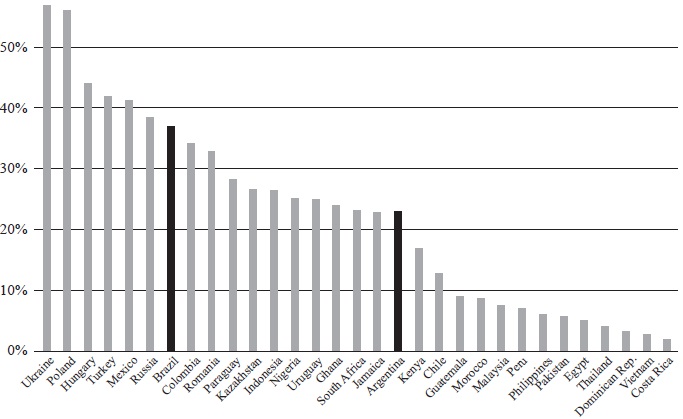
Source: IFS (IMF).
Figure 1 Depreciation of the nominal exchange rate vis-a-vis USD (August 2008-March 2009) for selected emerging economies.
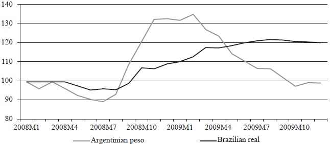
Source: IFS (IMF).
Figure 2 Nominal exchange rates of the Argentinian peso and the Brazilian real, 2008-2009. Indexed (2008M1 = 100), end-of-month data.
The Global Financial Crisis and its effects on other countries and currencies have been studied extensively, with different findings. Rose and Spiegel (2011) find that countries with current account surpluses seem to suffer less from slowdowns. Fratzscher (2009) finds that countries with low foreign reserves, weak current account positions and high financial exposure vis-a-vis the USA experience larger currency depreciations. Frankel and Saravelos (2012) select a wide range of variables from the Early Warning System (EWS) literature and find that international reserves and real exchange rate overvaluation are the most important leading indicators of the 2008-2009 crisis.
We approach the currency crises from an Early Warning System (EWS) perspective. We design a parametric model that issues signals or warnings well ahead of a potential currency crisis. The dozens of EWSs that have been developed differ widely in the definition of a currency crisis, the period of estimation, data frequency, the countries included, the inclusion of indicators, the forecast horizon, and the statistical or econometric methods used. For extensive overviews, see Kaminsky et al. (1998) or Abiad (2003). Boonman, Jacobs and Kuper, et al. (2014) focus on Mexico and find that the currency crisis in 2008 is not predicted by the EWS estimated with data from previous currency crises. We extend the methodology to Argentina and Brazil, the two largest South American countries, which have experienced several currency crises since the early 1990s. Both countries are considered emerging economies, have moved from fixed to floating exchange rate regimes, have a high dependence on commodities (although different commodities), and have been relatively open economies for trade and investment. Bilateral trade is high between Argentina and Brazil, and there has been contagion between the countries.
The majority of the EWSs is estimated for a panel consisting a large number of emerging economies. With its rich history of financial crises (Reinhart and Rogoff, 2009), empirical research on currency crises in Latin America has surged since the late 1990s. Herrera and Garcia (1999) construct an EWS that contains the real effective exchange rate, domestic credit growth in real terms, the ratio of M2 to international reserves, inflation and a stock market index in real terms as regressors; they apply their model to eight Latin American countries. They acknowledge that including external interest rates, commodity prices and the state of the real economy will probably improve the performance, but that this will add to the complexity of the model. They hint the use of factor models.
Argentina’s long history of currency crises and other financial crises is analyzed in several studies. Kaminsky et al. (2009) use a Vector Autoregression (VAR) model to quantify the role of domestic and external shocks in currency crises. They analyze Argentina’s currency crises from 1970 to 2001 and find that the crises have different causes. In some crises domestic fundamentals matter, in particular inconsistent monetary and exchange rate policies. Typically these policies are accompanied by hyperinflation, confiscations of bank deposits, and price and wage controls, which cause uncertainty and risk aversion of households and foreign investors. In other crises external indicators such as monetary tightening in industrial countries are key variables: the resulting capital flow reversals lead to currency crises. Contagion also plays a role in some crises in the 1990s. Alvarez-Plata and Schrooten (2004) apply the signal approach of Kaminsky et al. (1998) and find that the leading indicators could not have foreseen the Argentinean currency crisis of 2002. They suggest that in future research institutional indicators such as political turbulence and corruption be included. Cerro and Meloni (2013) analyze Argentina’s crises from 1865 to 2002. They use different techniques, including a multinomial logit model to distinguish mild and deep crises from very deep crises. They find that increases in public expenditures and government debt, as well as abrupt falls in the rate of growth of bank deposits are related to currency crises. Very deep crises are related to unfavorable external and domestic conditions. Toshniwal (2012) identifies common features in the financial crises that Brazil has experienced between 1982 and 2002. The country has ran large, unstable budget deficits that result in a high, unsustainable level of public debt and limited policy flexibility during economic crises. Also, Brazil has suffered from a structural high inflation leading to high interest rates. To fight the high inflation currency pegs and even new currencies have been used, but these have led in most cases to currency crises. Furthermore, a lack of political consensus on macroeconomic management and weak banking regulations have resulted in banking crises.
We investigate if currency crises from the period 1990-2007 contain information that is useful to predict the currency crises during the GFC (2008-2009) for Argentina and Brazil. We focus on the period since the early 1990s, because of data availability and because of the significant break with the periods of hyperinflation and the remains of inward-looking economic policies. The debt restructuring (Brady plans) and successful reforms to eliminate hyperinflation in Argentina (1991) and Brazil (1994) mark the start of this period. We model the probability of a currency crisis in an ordered logit model to account for the severity of currency crises. We distinguish three classes of currency crises (mild, deep and very deep crises) and tranquil periods (periods in which no currency crisis took place). We estimate the model and analyze the outcomes for each country independently. We include a large number of possible crisis indicators, based on the three generations of currency crisis models. Our choice to include a wide range of variables instead of preselecting explanatory variables is inspired by Kaminsky (2006) who emphasizes that there are many different causes. We use a static factor model to cope with the large number of crisis indicators. We estimate the factor models and the ordered logit models up to and including 2007, and present forecasts for the period 2008-2009.
We find that our model predicts the currency crisis in 2008-2009 in Argentina and Brazil reasonably well, in particular for Brazil. We interpret this result as follows. Currency crises that have occurred in the period up to 2007 contain information that is useful for predicting the currency crises in the GFC. This is in contrast to the common opinion that the GFC is not comparable with earlier crises. We see similarities and differences in the run-up to currency crises between the periods 1991-2007 and 20082009. Similarities consist of the sudden stop in capital flows, drops in commodity prices and a slowdown in international trade, which can be considered external causes (Kaminsky et al., 2009). This could explain why our model performs better for Brazil: most currency crises in Brazil between 1994 and 2007 originate from outside the country, similar to the currency crisis in 2008-2009. Differences are that the situation in the banking sector and the government (fiscal deficit, debt) is more sound in 2008 than in years prior to earlier currency crises, and that the crisis originates in a developed country. There are also differences between Argentina and Brazil at the time of the GFC. While Argentina has a low level of foreign investments and capital flows, Brazil has high capital inflows and its currency is considered overvalued. This could be a second explanation for the better performance of our model for Brazil.
This paper is structured as follows. Section “Methodology” discusses our method. The data and brief descriptions of the Argentinian and Brazilian crises are presented in Section “Data and background”. Section “Empirical results” presents the empirical results and the analysis of out-of-sample performance, followed by the conclusion.
Methodology
We first apply factor analysis to extract the factors from a large set of indicators, then use the estimated factors as regressors in the ordered logit model, with a crisis dummy as dependent variable, and lastly compute ex ante forecasts. Before we turn to these models, we first discuss crisis dating.
Crisis dating
We use the speculative pressure approach, inspired by Girton and Roper (1977), and later adopted by Eichengreen et al. (1995) for currency crises. This approach does not only take into account actual devaluation or depreciation of the currency, but also includes periods of great stress of the exchange rate. The approach is considered better than the successful attack approach, because it works well under both fixed and floating exchange rate regimes (Frankel and Saravelos, 2012). We follow the Exchange Market Pressure Index (EMPI) of Kaminsky and Reinhart (1999) defined as the weighted average of exchange rate changes and reserve changes, with weights such that the two components of the index have equal conditional volatilities. Kaminsky and Reinhart (1999) identify a crisis when the observation exceeds the mean by more than three standard deviations. We use this criterion to identify “very deep” crises. Similar to Cerro and Meloni (2013) we extend the crisis definition by introducing “deep” crises (which we define as two adjacent months exceeding between 2 and 3 times the standard deviation) and “mild” crises (which we define as two adjacent months exceeding between 1 and 2 times the standard deviation). The ordinal variable that indicates crises periods is constructed as follows: the value 0 indicates no crisis period, the value 1 is assigned to mild crises, 2 to deep crises and 3 to very deep crises. As is common in the literature, all crises identified by the EMPI definition are compared to the narrative and adjusted where necessary, for example when a large drop in the reserves is not used to defend the currency but to pay off debt (Brazil in 2000 and Argentina in 2005).
As is common in EWSs of currency crises, we assign the same dummy variable value for the run-up period to the crisis. Kaminsky et al. (1998) use a run-up period of 24 months with the argument that for policy makers the run-up period should be sufficiently long to be able to implement policies to avoid a crisis. Eichengreen et al. (1995) use a window of 2 quarters, while Bussiere and Fratzscher (2006) use a 12 months window exclusion period. We have used three different run-up periods: 6, 12 and 24 months. If depths of crises overlap we assign the highest ordinal number to that crisis.
The Static Factor model
We use the Static Factor model to avoid pre-selecting indicators, because we want to capture several crisis mechanisms. In factor models an observable set of N variables is expressed as the sum of r common components (factors) and the idiosyncratic component. The primary reason for the popularity of factor models is that one can include a large number of variables and let the model reduce this into a much smaller number of factors (N>>r). In the static, approximate factor model the idiosyncratic components are (weakly) correlated, which covers cross-correlation and heteroskedasticity between the idiosyncratic errors and correlation between the common components and the idiosyncratic components (Barhoumi et al., 2010). The principal components method can be used to estimate the factors.
One of the issues in factor analysis is the determination of the optimal number of factors. Various procedures have been proposed, such as the Bayesian Information Criterium, the Kaiser Criterium and Cattell’s scree test. With the large dimensional factor models of recent years many studies have proposed solutions and consistent estimators for the number of factors using different factor models and distributional assumptions. Here we employ the criterion of Otter et al. (2014), which is associated with Onatski’s (2009) test statistic, and related to the scree test. The criterion looks for the number of eigenvalues for which the difference between adjacent eigenvalueeigenvalue number blocks is maximized. The criterion outperforms other criteria including the Edge Distribution estimator of Onatski (2009), except for large samples (more than 300 variables or observations).
Using factor models comes at a cost. Determining the economic relevance of factors and interpreting the factors in a meaningful way is problematic. Many indicators enter in more than one factor, so focusing on a single factor only partially explains the full impact of an indicator on the probability of a crisis, and may even lead to counterintuitive results. In this paper we abstain from interpretation of the explanatory variables.
Ordered logit model
We use the ordered logit model to be able to distinguish in crisis severity. Severe crises have a different run-up than milder crises. Our dependent variable can take four values: no crisis, mild crisis, deep crisis, and very deep crisis. We employ an ordered choice model, which extends the binary choice model, allowing for a natural ordering in the outcomes y. An alternative is to use the EMPI as the dependent variable, instead of transforming it into four categories with the thresholds, then using a (linear) regression model. However, since there are far more tranquil periods than periods with crises, the model will be biased towards indicators that explain the EMPI in tranquil times. Additionally, crises are non-linear by nature: often a small change can trigger a crisis. The logit model captures that better than the linear regression model. We use the logit model, because the logistic distribution (logit model) has wider tails than the normal distribution (probit model). This is preferable if an event has a very low frequency, as is the case with financial crises (Manasse et al., 2003).
Most institutional variables that we use have low variation. When there is limited overlap in the values of (a set of) explanatory variables and the outcomes of the dependent variable, the regressions yield large estimates and standard errors. This problem is called quasi-complete separation (Zorn, 2005), and we avoid it by adding (a subset of) institutional and political variables to the factors as separate regressors.
Ex ante forecasts
The models are estimated using data up to and including 2007, and we test the out-ofsample performance of the estimated models for the period 2008M1-2009M12. We forecast the probabilities of a mild, deep and very deep crisis with our ordered logit model. We use realized monthly data for the indicators for the years 2008 and 2009, and extrapolate the factors without re-estimating the loadings of the static factor model.
We use the quadratic probability score (QPS) proposed by Diebold and Rudebusch (1989) to evaluate the out-of-sample forecasts. This measure indicates how close, on average, the predicted probabilities Pt and the observed realizations Zt are. The QPS is given by
The QPS achieves a strict minimum under the truthful revelation probabilities by the forecaster. In addition, QPS is the unique proper scoring rule that is a function only of the discrepancy between realizations and assessed probabilities. The QPS ranges from 0 to 2, with a score of 0 corresponding to perfect accuracy if the estimated probability is 1 (0) and a crisis does (not) occur for all t. A score of 2 shows that the model indicates a perfect false signal in which the estimated probability is 0 (1) and a crisis does (not) occur for all t.
Data and background
Our sample starts in the early 1990s, after the effects of spillovers of the 1980s Latin American debt crisis have faded out and when hyperinflation has been overcome. The analysis for Argentina starts after the introduction of the Convertibility Plan (April 1991) and for Brazil after the introduction of the Real Plan (July 1994), which both can be regarded as a break with the hyperinflation periods.
We estimate the Exchange Market Pressure Index (EMPI) based on the period up to December 2007, and extend this to December 2009. For the weights we use the standard deviations from the period up to and including December 2007.
Currency crises in Argentina and Brazil, 1990-2007
Both Argentina and Brazil have experienced several currency crises in the period 1991, resp. 1994 to 2007. Graphs of the currency crises (employing a 12 months run-up) are plotted in Figures 3 and 4.
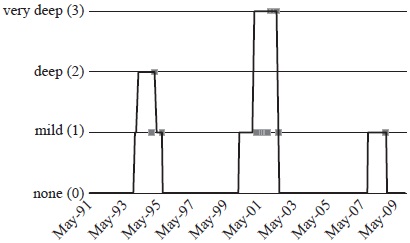
Notes: The squares correspond to the months of the currency crisis. The line includes a 12 months run-up period for each crisis.
Source: Own elaboration.
Figure 3 Currency crisis episodes for Argentina for the period 1991-2009, with a 12 months run-up period for each crisis.
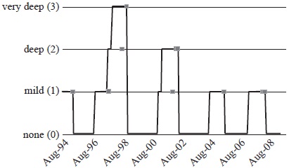
Notes: The squares correspond to the months of the currency crisis. The line includes a 12 months run-up period for each crisis.
Source: Own elaboration.
Figure 4 Currency crisis episodes for Brazil for the period 1994-2009, with a 12 months run-up period for each crisis.
Argentina experiences a currency crisis in 1995, which is related to the “tequila crisis” in Mexico. Argentina’s banking system suffers from large deposit withdrawals, as rumors spread that systemic banks may fall due to their exposure to sovereign debt. In March 1995 the peg is successfully defended through the use of reserves and interest rate. This event is considered the first currency crisis of the Convertibility Plan that was launched in April 1991 (Kaminksy, Mati and Choueri et al. 2009). In 2001 the international capital markets are still wary of emerging economies (Asian, Russian, LTCM, Brazilian and Turkey crises). Domestically the political uncertainty and the financial turmoil following Brazil’s crisis in January 1999 has severely affected private investment and consumption in Argentina. The country is stuck with twin deficits, a trade gap and a budget gap, that foreigners are less and less willing to finance (Economist, 2005). In December 2001, the government defaults on its debt, and in January 2002 the currency peg to the dollar is released, and rapidly loses value. The banking sector collapses, due to its high exposure on sovereign debt and the high default rate of the private sector in the face of the crisis, making it a triple crisis (Guidotti and Nicolini, 2016).
Brazil experiences a currency crisis in 1995, caused by the contagion from the “tequila crisis”. Similar to Argentina, Brazil is able to defend the peg by increasing interest rates and using reserves. In 1997 Brazil comes under pressure with the Asia crisis. The Brazilian currency is overvalued by up to 40%, the commodity prices drop, increasing the current account deficit, which is financed by borrowing in the external capital markets (Gallo, 2006). The currency can be defended, but at the cost of the use of reserves. However, the pressure returns with the Russia crisis in the fall of 1998, and in January 1999 the currency is floated and rapidly depreciates. The IMF has to step in to avoid a sovereign default, but the healthy and well-regulated banking sector is not in danger at any time (Gruben and Welch, 2001). In 2002 the country is hit again; global uncertainty due to the Argentina 2001-2002 crisis combined with political uncertainty on the new presidents’ economic policies lead to a strong depreciation of the Brazilian real in July and September 2002. A large IMF loan helps to restore confidence, and to avoid a debt default (Toshniwal, 2012). In December 2005 the real depreciates and the reserves drop sharply; the situation reverses in the months thereafter.
Argentina and Brazil in 2008-2009
In the run-up to the crisis in the fall of 2008 both Argentina and Brazil experience a period of economic prosperity in the 2002-2007 boom, featuring large foreign reserves, small sovereign external debt levels, small fiscal deficits (or even surpluses), and a more flexible exchange rate regime. But there are differences too. Brazil faces a strongly appreciated currency before the onset of the crisis and an unprecedented large amount of foreign reserves (Ocampo, 2009). For Argentina key economic conditions are less favorable, in particular the high and persistent inflation, which reflect important macroeconomic imbalances (Rojas-Suarez, 2011). In addition, the central government debt is higher than in other Latin American countries (Ocampo, 2009), as well as the ratio of short-term external debt to international reserves (Rojas-Suarez, 2011). Political risk increases, because of its macroeconomic and debt-servicing policies (Porzecansky, 2009), the anti-globalization policies that it shares with Ecuador and Venezuela (Rojas-Suarez, 2011), and through government’s decisions such as the nationalization of its private pension regime in late 2008.
In the fall of 2008 both countries experience a currency crisis, considered a mild crises according to our definition. The Brazilian real depreciates more and faster than the Argentinian peso. Both countries are hit by an unusually heavy drop in export earnings between the fourth quarter of 2008 and the first quarter of 2009. Brazil is hit by a second exogenous shock: heavy reversals in capital flows in the fourth quarter of 2008. Surprisingly, Brazil does not experience a major financial crisis, or even a worsethan-average deceleration in economic growth (Porzecanski, 2009). During the crisis Brazil implements both counter-cyclical fiscal and monetary policies (Rojas-Suarez, 2011). In 2008 economic conditions prevent Argentina to undertake counter-cyclical monetary policy, but it implements counter-cyclical fiscal policy. Rating agencies downgrade Argentinian government bonds and the spread surge to even higher values than during the 2002 crisis. The institutional environment does not help to deal with the crisis. The elections scheduled for October 2009 are held in June 2009 in order to deal with the GFC. However, the outcomes of the elections makes things worse for the ruling president’s party which loses its majority in parliament.
Data and sources
For the explanatory variables we select the “usual suspects” (the common macroeconomic and financial variables), institutional and political variables, commodity-related and global indicators. The selected indicators can be classified into separate categories:
13 external economic indicators, among which the deviation from real exchange rate trend, exchange rate volatility, growth of exports, imports and foreign reserves, import cover, ratio of M2 to foreign reserves.
17 domestic economic indicators, among which domestic real interest rate, inflation, M2 multiplier, industrial production, share market index return.
14 institutional and political indicators, among which Herfindahl indices, political stability, corruption, investment profile, internal conflict, election years.
10 debt indicators, among which total debt, short term debt, debt service, arrears.
11 banking sector indicators, among which credit to public sector, to private sector, ROE, deposits.
5 global and regional indicators, among which world economic growth, US yield, contagion dummy.
12 commodity related indicators, among which prices of oil, metals, agricultural products, exports and imports of fuel, agricultural products, food and metals as percentage of GDP.
The main sources for the data are the International Financial Statistics (IFS) database of the IMF, the World Development Indicators (WDI) from the World Bank, International Country Risk Guide (ICRG) database of the Political Risk Services Group, and Beck, Demirguc-Kunt and Levine et al. (2009).
Some data limitations exist. Not all time series are sufficiently long which limits the selection of explanatory variables. A particular issue is the exchange rate regime. Both countries have moved from a controlled exchange rate regime to a more freely floating regime after a major crisis hits the country (Ilzetzki, Reinhart and Rogoff et al. 2008). With an already low number of crisis observations it is complicated to further disaggregate data by distinguishing exchange rate regimes. Additionally, the variation of the regime changes is very low, which leads to the problem of quasi-complete separation (Zorn, 2005).
The series have been tested for non-stationarity (using Augmented Dickey-Fuller tests) and visually inspected for seasonal effects. Where necessary a transformation is made to render them stationary. To deal with mixed frequencies in series, we apply simple quadratic interpolations. All series are normalized, i.e. demeaned and divided by its sample standard deviation.
Empirical results
We estimate the ordered logit model for Argentina and Brazil for the period up to and including 2007 using a run-up period of 12 months, which is shown in Subsection “Regressions”. In “Forecast performance” we use the estimated model to predict out-of-sample. In “Robustness checks” we present robustness checks, using a 6 and 24 months window exclusion period.
Regressions
Argentina. The criterion of Otter et al. (2014) suggests 10 factors for Argentina. In Table 1 we present estimation results. We do not attempt to interpret the factors for reasons we explained in Subsection “The Static Factor model”. The institutional and political indicators are briefly interpreted. A higher level of internal conflict and an election year (for legislative power) are associated with deeper currency crises. The latter can be explained by the political economy theory that shows that governments prefer to postpone painful decisions (including the devaluation of an overvalued currency), and a new government may see no way out then to devalue. The first result seems at odds with intuition. A possible explanation can be found in the third generation currency crisis models, combined with elements from boom-bust and sudden-stop models. When institutional conditions improve, expectations increase, and investments increase. This attracts foreign capital and leads to a capital account surplus. Additionally, the high expectations may lead to overlending and overborrowing, thus creating a bubble in debt and other asset prices. When the expectations decrease, foreign investors withdraw their investments, thus causing a sudden stop in capital flows. As a consequence, the pressure on the exchange rate to depreciate increases.
Table 1 Ordered logit estimation results for Argentina 1991M5-2007M12, with a 12 months run-up period.
| Coefficient (standard error) | Coefficient (standard error) | ||
|---|---|---|---|
| SF1 | -0.269 (0.121)** | SF8 | 0.167 (0.219) |
| SF2 | -0.406 (0.114)*** | SF9 | -0.376 (0.183)** |
| SF3 | 0.341 (0.174)** | SF10 | 0.234 (0.271) |
| SF4 | 0.215 (0.104)** | ∆ (INTCONFL) | 1.074 (0.235)*** |
| SF5 | -1.252 (0.247)*** | ∆ (LAWORD) | 0.542 (0.380) |
| SF6 | 0.064 (0.183) | ELECLEGYR | 1.048 (0.530)** |
| SF7 | 0.847 (0.193)*** | Adjusted pseudo R2 | 0.411 |
Notes: *: significant at 10%, **: significant at 5%, and ***: significant at 1%;
Explanations of the symbols used: SF1: Static Factor 1, SF2: Static Factor 2, et cetera; ∆ (INTCONFL): Change in internal conflict dummy variable (increase implies less internal conflict, or a lower risk); ∆ (LAWORD): Change in the law and order dummy variable (increase is improvement in law and order, representing a lower risk). Includes the strength and impartiality of the legal system and law enforcement; ELECLEGYR: Dummy variable that is 1 if there is an election year for the legislative power and 0 otherwise.
Adjusted Pseudo R2: Coefficient of correlation for the ordered logit regression model, adjusted for the degrees of freedom.
Source: Own elaboration.
Brazil. For Brazil the Otter et al. (2014) criterion suggests 8 factors. The institutional and political indicators that are significant and do not cause quasi-complete separation are bureaucratic quality and law and order. While an improvement in bureaucratic quality is associated with a lower probability of currency crisis, an improvement in law and order conditions is associated with a higher probability of currency crises. The first is in line with expectations, but the latter seems to be counter-intuitive. This may be explained by the same mechanism as described for Argentina.
Forecast performance
In this section we investigate the out-of-sample performance of the estimated models in the period 2008M1-2009M12.
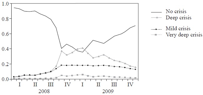
Argentina. The out-of-sample performance of our EWS model for Argentina is shown in Figure 5. The probability of no crisis decreases steadily since the beginning of 2008. In September 2008, the month of the Lehman Brothers event, the probability of no crisis is still 75%, while the probabilities of a mild and a deep crisis sum up to 25%. In 2009 the probability of no crisis continues to decline and is close to zero by the end of 2009. The probability of a deep crisis continues to increase in 2009.
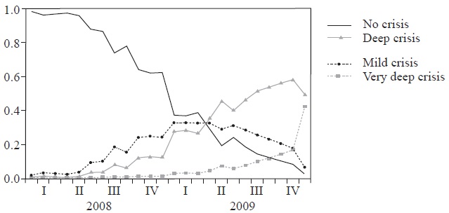
Source: Own elaboration.
Figure 5 Argentina: probability of crisis and no-crisis for out-of-sample period, 2008-2009.
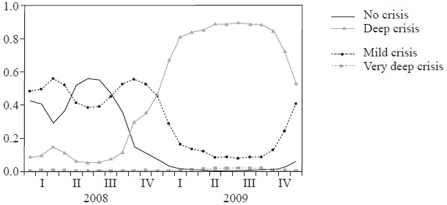
Brazil. Figure 6 shows the out-of-sample performance of our EWS model for Brazil. The graph shows a modest increase in the probability of a crisis in the run-up to the mild currency crisis that initiated in September 2008. The probability of no crisis decreases rapidly after September 2008. In the same period the probability of a deep crisis rises to reach 70%. In reality a mild currency crisis occurs.
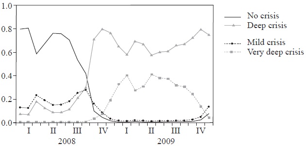
Source: Own elaboration.
Figure 6 Brazil: probability of crisis and no-crisis for the out-of-sample period, 2008-2009.
Complementary to the graphic representations in Figures 5 and 6, we use the Quadratic Probability Score (QPS) to evaluate the probability of a crisis out-of-sample (2008M1-2009M12) for mild, deep and very deep crises. In this period Argentina and Brazil experience a mild crisis. We show the results in Table 3.
Table 2 Ordered logit estimation results for Brazil 1994M8-2007M12, with a 12 months run-up period.
| Coefficient (standard error) | Coefficient (standard error) | ||
|---|---|---|---|
| SF1 | 0.243 (0.049)*** | SF7 | 0.589 (0.125)*** |
| SF2 | -0.318 (0.079)*** | SF8 | 0.433 (0.127)*** |
| SF3 | 0.168 (0.064)*** | ∆ (BURQUAL) | -1.441 (0.319)*** |
| SF4 | -0.048 (0.081) | ∆ (LA WORD) | 1.336 (0.293)*** |
| SF5 | -0.627 (0.108)*** | Adjusted pseudo R2 | 0.287 |
| SF6 | -0.085 (0.111) |
Notes: *: significant at 10%, **: significant at 5%, and ***: significant at 1%;
Explanations of the symbols used: SF1: Static Factor 1, SF2: Static Factor 2, et cetera; ∆ (BURQUAL): Change in the bureaucratic quality dummy variable (increase is improvement in bureaucratic quality, or lower risk). High quality when the bureaucracy has the strength and expertise to govern without drastic changes in policy in government service; ∆ (LA WORD): Change in the law and order dummy variable (increase is improvement in law and order, representing a lower risk).
Adjusted Pseudo R2: Coefficient of correlation for the ordered logit regression model, adjusted for the degrees of freedom.
Table 3 Out-of-sample performance of logit models with 12 months run-up, using the Quadratic Probability Score (QPS).
| Country | Mild | Deep | Very deep |
|---|---|---|---|
| Argentina | 0.778 | 0.200 | 0.022 |
| Brazil | 0.627 | 0.606 | 0.100 |
Source: Own elaboration.
Recall that the closer the score statistics in Table 3 are to zero, the more accurate the model predictions are. A value of 2 indicates a perfect false signal. Our EWS model performs reasonably well for Argentina. The QPS for the actual crisis severity (mild crisis) is 0.778. With a score closer to zero than to two, we interpret this as a reasonable, yet not highly accurate model prediction. The scores are much lower for the probabilities of a deep crisis and a very deep crisis, which means that our model predicts well that there is low probability of a deep or very deep crisis. In Figure 5 we observe that the probability of a currency crisis increases in 2008. Both mild and deep crises show an increased probability.
The outcomes for Brazil are similar to the outcomes for Argentina. The model performs better for predicting the correct severity of a crisis (mild crisis), as the QPS is lower (0.627), but it performs worse for identifying a deep and very deep crisis, as the QPS are higher than for Argentina (0.606 versus 0.100). According to our definition the crisis in Brazil is a mild crisis, but the EMPI is very close to the threshold that would identify it as a deep crisis. This is also visible in Figure 6, where the probabilities of a mild crisis and a deep crisis increase equally in the run-up to September 2008. We conclude that our EWS does a reasonably well job in indicating a currency crisis for Brazil, although it indicates a more severe crisis than actually occurred.
Comparing the performance of our model to the actual outcome, we observe that predictions for Brazil are better than Argentina’s predictions. The predicted probability of a crisis in Brazil increases rapidly in 2008 (Figure 6), in a faster pace than the probability of a crisis in Argentina (Figure 5). Our model does not differentiate well between a mild and a deep crisis, which seems natural as the crisis is near the threshold that distinguishes mild from deep crises. Also the QPS is lower for Brazil than for Argentina. We provide several explanations for this difference. First, Brazil has experienced more currency crises in the in-sample period than Argentina did. Therefore, the model has identified better for Brazil which indicators play a role in the crisis runup. Second, the countries are different in openness and capital flows in the run-up to the currency crisis of 2008-2009. The Argentinean economy is relatively closed for foreign capital and investments because of the political situation and the ongoing sovereign debt crisis negotiations related to the 2001-2002 crisis. Brazil’s currency is considered overvalued and capital inflows are high.
Robustness checks
We also perform the analysis for two alternative run-up periods. An Early Warning System with a run-up period of 12 months may be too short for the authorities to implement policies to avoid a currency crisis. An Early Warning System with a run-up period of 6 months is likely to be more accurate as indictors will show special behavior as a crisis is approaching. The results for the models with a 6 and 24 months run-up period are shown in the Appendix and are discussed below.
Contrary to findings of Kaminksy (2006) we find that the model is sensitive for changes in the length of the run-up period. The fit of the regression during the insample period differs from one run-up period to the other, as shown in Tables 4 and 5 of Appendix A.1. For Argentina the fit of the 6 months run-up model (measured by the adjusted pseudo R2) is higher than the 12 and 24 months run-up periods. For Brazil the contrary applies, the fit is better for the model with a long run-up than for a short runup. We interpret these findings as follows. Currency crises in Argentina tend to develop fast, while currency crises in Brazil develop at a slower pace.
For the forecasted period (2008-2009) the results are more homogenous, as shown in Figures 7 to 10 in Appendix A.2. For both countries the model with a 24 months runup signals crises earlier and more pronounced than models with a 6 or 12 months runup. As in the 12 months run-up case, Brazil shows a better performance than Argentina in the out-of-sample period.
Conclusion
The financial panic that follows the fall of Lehman Brothers in September 2008 affects many countries and regions including Latin America. In Brazil the exchange rate depreciates by more than 40%, the Argentinian peso depreciates by 25% and financial markets (stocks, bonds) are hit hard. This paper investigates the experience of the two biggest South American countries with currency crises since the 1990s, and whether the currency crisis in 2008 could have been foreseen -despite the common opinion that the GFC has very distinct features than earlier crises, which makes it impossible to compare with earlier crises.
We develop an Early Warning System for currency crises since the early 1990s up to 2007. We develop an EWS consisting of an ordered logit model, using static factor models to reduce the dimension of the information set. We use our EWS to forecast the probability of currency crises in 2008 and 2009. Our model predicts the currency crises in the fall of 2008 for Argentina and Brazil, although the predicted crises are more severe than actually occurred. We conclude that the currency crises in 1991-2007 contain information that is useful for predicting the currency crisis in 2008-2009. Our model performs better for Brazil than for Argentina, which we attribute to (i) more crisis observations in Brazil imply a better model fit, which is favorable for predicting crises and (ii) Argentina’s economy is relatively closed prior to the GFC while Brazil’s economy is more open.