Introduction

In the economic literature, there are several indices that intend to capture the wellbeing of individuals. Some capture differences in income, health conditions, capital, productivity, welfare, etc., among human groups with common attributes. Some others try to measure external variables such as environmental quality. Most indices offer some information on how individuals or groups compare to each other. From the Human Development Index to the Environmental Protection Index, all indices are relatively sound with a theoretical background. These constructions are important for policy analysis and public decision making in many areas.

In this paper we offer a simple estimation of the Quality of Life Index (QLI) for Mexican cities, which is an empirical application of the theory of equalizing differences, formalized by Rosen in 1976 based on previous work on hedonic prices. The important assumption under this QLI comes from the idea that individuals may be willing to pay or give up some part of their money income, for amenities they value more. From this view, quality of life is related to the value of external amenities attached to visible prices in the market. These amenities may come in the form of clear air, clean water, safe neighborhoods, access to local public goods, quality of education and health care, etc. It is difficult to accept that individuals ignore these amenities when making the important decision on where to live and work. Although there are many other important considerations to take into account about locational decisions of households and firms, QLI offers a first-hand measure of the relative importance of environmental and social amenities (or disamenities)

This analysis is perhaps, to the best of the author’s knowledge, the first Quality of Life Index constructed for Mexican cities using hedonic prices approach. Although this methodology was developed more than three decades ago, there is almost no literature in the subject for Latin American countries. Another important structural change since its development is the advance of federalism and devolution of fiscal attributes from central to local governments. The new relation between levels of governments has increased the bundle of local public goods available and so the positive (or negative) externalities derived from them. In this context, the QLI acquires a new relevance as a useful tool for understanding qualitative differences among regions and cities.

The QLI is just a weighted average valuation of an amenity bundle in each region or city. The construction of QLI requires first the estimation of implicit prices for every amenity (disamenity), then it uses these implicit prices and the average amenity provision in every city to obtain the value of the amenity bundle. It offers information on how these amenities are valued by the average household in every city compared with other cities. Then the relevant questions are the finding of the appropriate micro-data and the proper estimation of the implicit prices.

The Quality of Life Index using the approach of equalizing differences was first developed by ^{Rosen (1979)} and later refined by ^{Roback (1982)}. Since then, several authors constructed on these works and developed different models to estimate QLI adding new relations with different spatial coverage. Examples are ^{Gyourko et al. (1991)} which is a QLI construction for US that includes taxes and public goods; ^{Colombo, et al. (2012)} is a QLI construction for Italy; ^{Albouy, et al. (2013)} is a QLI construction for Canada which includes cities’ productivity; Berger, et al. (2007) is a QLI for Russia and ^{Zheng, et al. (2009)} is a QLI for China. They all use hedonic prices approach and estimate wage and housing differentials.

Forwardness of the ^{Roback’s model of 1982}. The simplicity is justified by the reality of Mexican Municipalities (cities), which are limited to the use of property taxation and are highly dependent on federal grants as a main source of revenue. The basic administrative structure in Mexico is the Municipality, which in many cases includes many cities of different size. We are separating those municipalities where there is a city with more than one hundred thousand inhabitants. In many cases, these cities make up the entire municipality, so the concept of city is used in this paper instead of municipality.

The paper uses official data sets from the Mexican National Institute of Statistics, Geography and Informatics (INEGI). Household characteristics come from the Mexican National Household Income and Expenditure Survey (ENIGH) of 2010, while the information about local taxes, grants, and amenities come mainly from the State and Municipal Data Base System (SIMBAD), both supplied by the INEGI.

The ranking of Mexican cities within this new QLI is fairly consistent. Highly developed modern cities show high QLI. Most of these cities have strong economies, modern infrastructure and a large service sector, including tourist attractions like beaches, theatres, good hotels and resorts, etc. They also concentrate better health services, education and recreational facilities. These cities are usually connected toeach other within a metropolitan area so they share the spillover of local public goods and the economies of scale.

On the other hand, low QLI cities have serious urban problems relative to others. They also have many illegal urban sprawls, a difficult social network and larger crime rates relative to others. They also have lower provision of public goods and usually they benefit much less from spillovers and from being close to a metropolitan area.

In this work there are two different constructions of QLI using slightly different amenity bundles. One includes only local taxes and the other also includes federal grants. Both QLI rankings show some consistency though there are some changes in the ranking, especially in the top, due to unusually high grants for some cities, but the bottom of the ranking remains fairly unchanged.

This paper is organized as follow: The first section contains the introduction, the second the theoretical framework, the third contains two subsections to explain the data and the methodology for estimation, and the last contains our final conclusions.

Theoretical background

The idea of using the framework of equalizing differences to develop a QLI came back from ^{Rosen (1979)} and ^{Roback (1982)}. Consumers (workers) and firms face a bundle of amenities in specific geographical areas where wages, rents and amenities are in spatial equilibrium which means that there is no incentive to move. Gourkyo et al., 1991, introduced a model to incorporate taxes and local public goods. This section develops a simple model following Roback, 1979, and ^{Gourkyo, 1991}. The only difference is the addition of property taxation in the consumption of land services rather than include it only to the price of land. Local public goods are determined exogenously in the model. The reason for this comes from the fact that the Mexican fiscal revenue system is highly concentrated at the federal level and most local government revenue comes from federal grants.

In this world, location and transportation costs are ignored for both consumer and firms. Consumers are identical and derive utility from a composite private good x, a local public goods G, the consumption of residential land l and local amenities a. Consumers are identical in skills and tastes and supply one unit of labour. They also receive a salary income w and pay a property (local) tax⁡T. The price of the private good is normalized to one and the price of land is the rent r. They also receive a categorical grant g from the federal government and have a non-labour income of I. The consumer problem is to maximize the following utility function:

The above utility function includes the quality of local public goods in the same manner as local amenities. The budget constrain for the individual is:

The problem to the consumer is to maximize 1 respect to 2. From the above problem an indirect utility function can be obtained:

The firm’s problem is similar as in ^{Roback, 1982}, but property taxation is additionally included. Firms produce a X quantity of private goods using constant returns to scale production function. The relevant factors are land used for production lp and total labor N. The amenities bundle a enters the production function as follows:

The problem of the typical firm is to minimize costs subject to 4. The equilibrium condition is that unit cost must be equal to product price which is unity:

The standard conditions are Cw= NX and  Cr= lp(1+τ)X. If the amenity is unproductive then Ca < 0 and if the amenity is productive then Ca < 0. Industries may have an incentive to relocate to cities where productive amenities are available.

Finally, a simple local government budget constrain closes the system:

The grants g is positive because it is a transfer from federal government to local residents, then the total amount of public goods consumed are equal to the total amounts of grants and the local property tax collected. This also implies that local public goods are not always provided by local governments, which may be the case of Mexican Municipalities². It is clear from 3 and 5, that wages and rents are determined in equilibrium in both markets as functions of a. Finding the differentials from 3 and 5 and solving for dw/da and dr/da we find the wage and rental differentials as follow:

The above equations can be used to solve for Va, Vw and ca considering the conditions that Cw=NX and  Cr= lp(1+τ)X. A relative valuation can be obtained to measure the total amount of income required to compensate a household for a small change in a, which is called full implicit price IP:

The full implicit price of an amenity is the housing price differential dr/da and the negative of the wage differential dw/da. In principle, dw/da < 0 because wages must be adjusted downwards if there is an amenity. In this case, individuals are willing to give up some wage income to enjoy an amenity such as fresh air or safe public parks. We assume that the rent differential is dr/da > 0 because amenities make land (housing) expensive for households.

In the last equality, the parameter θ1 contains information on the total expenditure on net land consumption by households. The reader may also observe that dln⁡rda and dln⁡wda can be easily estimated using suitable data and appropriate statistical methods. Once these differentials are estimated for each amenity (disamenity) a vector of implicit prices for each amenity can be obtained IPai.

Using the vector of implicit prices IPai , a QLI can be easily constructed. QLI is the product of the implicit prices for each amenity by the average value of the trait in each city j:

(10)QLIj=∑i=1AIPijA-ij,where i = 1,...,Aand j = 1,..., J

Thus QLI can be interpreted as the money value that the average household assigns to the amenity bundle A in the city j. This QLI will be high for cities where amenities are highly valued and a simple ranking may be constructed for comparison.

Measuring Quality of Life

The data

Before proceeding to estimate the QLI, we must find suitable data for the experiment. It is often possible to find labour information and housing data in any household income-expenditure survey from any country. But it is unusual or extremely rare to find information about urban and environmental amenities within these types of surveys. So we must pool different data sets in order to input information on the amenities side by side with the labour and housing information.

The labour and housing data used in this work comes from the Mexican National Household Income and Expenditure Survey (ENIGH) of 2010 and information about amenities comes from the State and Municipal Data Base System (SIMBAD), both produced by the Mexican National Institute for Statistics, Geography and Information (INEGI). The ENIGH contains information from a sample of 27 thousand households representative for the whole country. The main variables used from this survey includes household income, characteristics of the head of the household, structural characteristics of houses, housing expenditure (rents), wage income and other labour market variables.

A subsample was constructed using household heads with a salaried work in the private sector, when the household is resident in a city with more than 100 thousand inhabitants. A total subsample of 7,966 households was obtained with enough number of observations to represent 92 middle sized and large cities. There are two main reasons behind the construction of this subsample. The first has to do with the concept of the QLI defined above, where we only include the valuation of households whose locational decision is decided by wages, rents and, of course, prices of amenities in every city. We are excluding those households that derive mainly income from capital and other non labour income as they may also do locational decision considering the productivity effects of amenities³.

We also decided to exclude household heads working in a public sector job as the public service in Mexico has some important institutional arrangements that may also affect locational decisions. Some individuals in public jobs may not be able to choose location like those in the military. Furthermore, almost all public workers are unionised and then willing to bargain wage hikes or other fringe benefits (e.g. support for rent payments) in places where there are highly-valued amenities for both households and firms. The effect of unionisation may be important especially in large cities. Due to possible rigidities in the labour market, we decided to exclude public workers in this analysis and leave these groups of workers for further research⁴.

The construction of the above subsample of private-sector salary workers is representative for the whole country. The objective is to make simple the empirical analysis as well as to fit properly the theoretical model. The main scientific objective is to obtain a vector of households’ valuations that may be used as weights to understand how these workers value local amenities. The vector IPai. contains the mean valuation of every amenity (disamenity) for the entire sample of private-sector and salaried workers.

These weights then can be used along mean values of the amenities (disamenties) to construct the QLI.

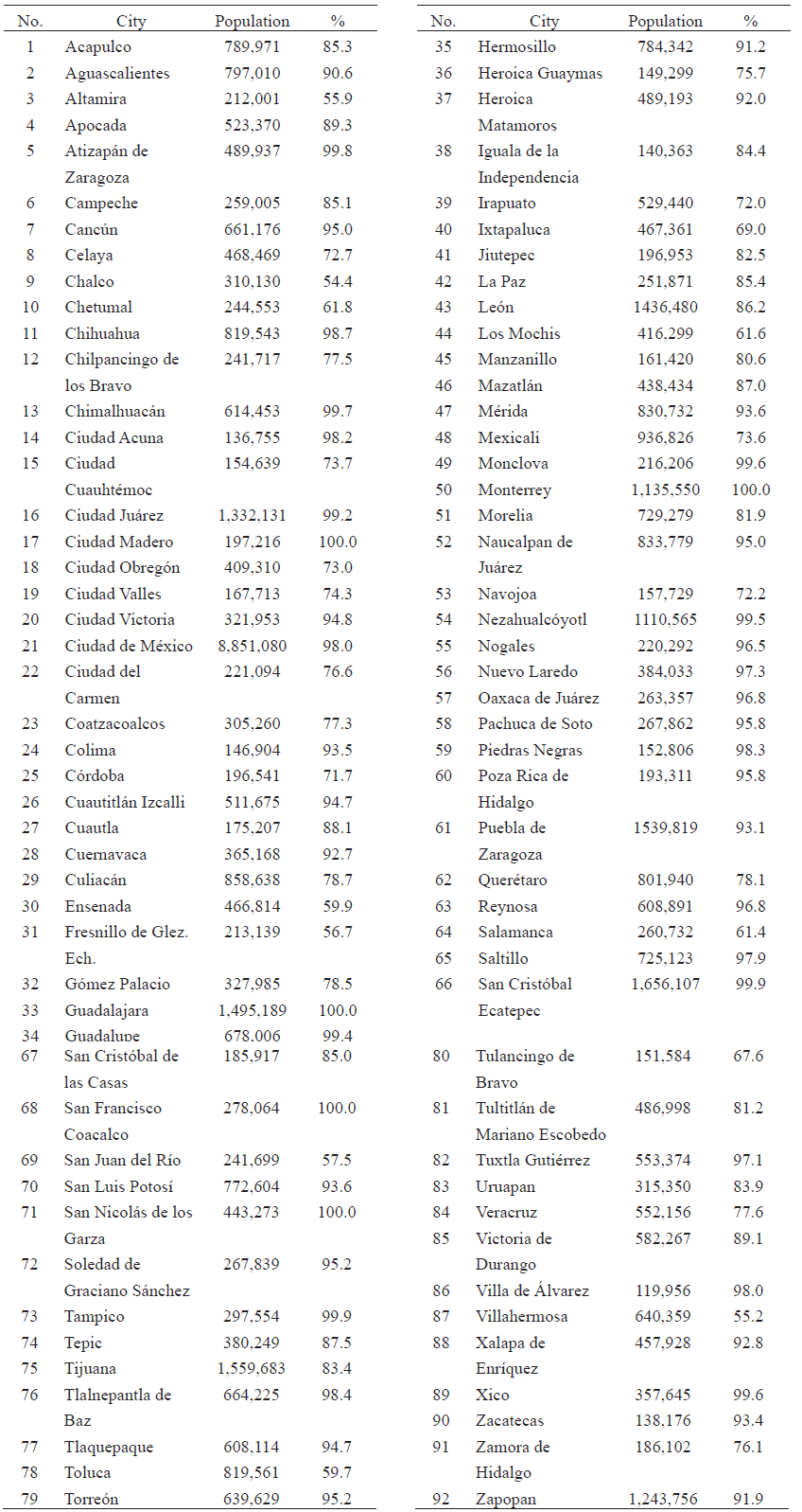
As mentioned before, there is no information at city level, so we used information at municipality level. In most cities, the total population is the same as the entire municipal population.Table 1 at the end of the paper shows the 92 main cities used for this analysis, with the total city population and the percentage from total municipal population. On average, city-level population represents 85% of the entire municipal population in this analysis.

Table 1: Relative size of main city population from the total municipality population 

Information on wages and rents were also obtained from the ENIGH. Wage income can be easily estimated for every member of the household and information on rents paid by the household is also included in the data sets⁵. In the survey, households were asked to provide an imputed value of rents for their estates (land and house), later we used this imputed rents as a proxy for market rents.

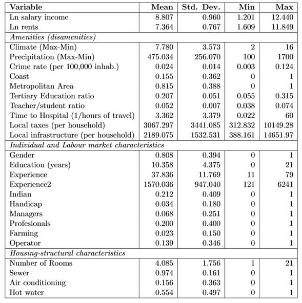
Information about amenities was obtained from the SIMBAD such as climate, precipitation, crime, education, health and fiscal attributes. Several data sets were constructed and later pooled to construct a unique data set with labour, housing and amenities information. Standard statistics of this data set are shown in Table 2 at the end of this paper.

Table 2: Standard Statistics 

Climate and precipitation data was used to capture the weather conditions in every city. A crime rate for every city was constructed dividing the total number of crimes by total population, in order to obtain a relative measure of public safety. Dummies variables were constructed to capture the advantages of being located next to the coast as well as the advantages of being located in a metropolitan area. These two variables also capture important aspects of urban agglomeration such as low transport cost, positive externalities of developed markets, among others.

In order to capture the quality effects of some local public goods provided by federal and state governments, a tertiary education ratio and a teacher-student ratio were constructed. These ratios provide also a good incentives for relocation and many households might also value the provision of tertiary education and the positive externalities of living close to well educated neighbours. The teacher-student ratio captures the intensity and also quality of primary education in every city.

The time-to-hospital variable accounts for the number of hours a family must travel to the nearest hospital in case of medical emergency. This variable was introduced in the regression as the inverse of the travel time to the nearest hospital which can be interpreted as a convenience or accessibility ratio. The average time of travel is about half an hour to the nearest hospital, but there are 9 households that declare more than 20 hours of travel, and five of these are located in Mexico city and from those, two declare taking up to 45 hours of travel even though these households are located inside the city. A possible explanation could be the segmentation in the social security in Mexico where some households might take a long travel time to arrive to their assigned hospitals.

The last two variables inside the amenity vector are Municipal taxes and local public goods provided by the city in the form of local public infrastructure. In Mexico, municipalities have few taxes at their disposal, and perhaps the most important is the property tax. This tax is a good instrument to observe the fiscal effort of every city as well as the provision of local public goods. One problem with local taxes in Mexico is that they only represent about 10% of the total municipal revenue. In order to properly include the quality-effect of local public goods provided by the city, federal grants must also be included in the analysis. One problem is that categorical grants were almost perfect collinear with local taxes as they are linked through a design formula. On the other hand, non-matching grants cannot be combined with categorical grants as they are not entirely committed to provide local public goods. So, a third variable was used to capture the effect of grants, particularly those categorical grants that are used to build local public infrastructure. If city fiscal revenue from taxes is small compared to grants, then it is possible to capture the effect of local public goods provided using the amount of investment in municipal infrastructure per household⁶.

Although the theory assumes that all households are identical, in practice we must control for workers’ heterogeneity. For that purpose, information about the head of household was used to capture individual-labour market characteristics such as gender, years of formal education, job experience, ethnicity and possible physical disabilities. Some dummy variables were used to capture information about industry level and labour market characteristics. These dummies captured information about types of jobs such as managers, machinery operators or professional jobs as well as jobs in agriculture.

Finally, a vector of structural housing characteristics contains information about the number of rooms in the house, and the availability of a sewage system and hot water inside the house.

The econometrics

The General Equilibrium Model implies that all markets (market goods, labour and land) are in equilibrium. But the market prices of interest that make for this equilibrium are, of course, wages and rents. Then we proceeded to estimate a reduced-form of wage and housing expenditures equations in order to estimate implicit prices as in 9. The functional forms follows standard Mincerian-type wage equations and housing equations which are common in the economic literature:

(11)ln⁡w = β0+ β1X + β2M + β3Z + ϵ, where ϵ∼N(0,σϵ2)

(12)ln⁡r = λ0+λ1Q + λ2Z+μ, where μ∼N(0,σμ2)

Where X is a vector of individual characteristics for the households’ heads, M is a vector of industry-level and labour market variables, Q is a vector of structural characteristics of housing, and Z is a vector of amenities. The vector of amenities Z was included to capture implicit valuation of non market goods and β3 and λ2 give an estimate of the wage and housing differentials in 9. If the amenities are statistically significant, then it is possible to offer a implicit price. Both 11 and 12 are explicit semi-log functional forms that follows the standard Mincerian and housing regressions. Another feature of these functional forms it is to allow for a straightforward estimation of the differentials in 9 ⁷.

The first approach was to perform traditional cross-section OLS regressions on 11 and 12 using the sample of 7,966 households. Several regressions were performed with different explanatory variables. We used information criterion (Akaike and Schwarz) in order to observe for the quality of the regression models. For the wage equation 11, we used 20 explanatory variables and for the housing equation 12 we used 14, from which 10 variables were included as amenities in the vector Z. As for this vector of amenities, we decided to include information on weather (temperature and precipitation), incidence of crimes as proxy of public safety, access to sea coast (seascape), metropolitan area (urban spillovers), tertiary and primary education index (university and teacher/student ratios), time to the nearest hospital in case of emergency, local taxes (property tax) and investment on local infrastructure (federal and state transfers).

As predicted by theory, almost all explanatory variables selected were significant, but a BreuschPagan and a White test reveal a serious problem of heteroscedasticity in the simple OLS regression⁸. A second OLS regression with robust standard errors resulted again with almost all explanatory variables being highly significant.

Correcting for heteroskedasticity does not solve all problems in our data. In our experiment, we are dealing with household information grouped by cities (municipalities) which brings into the picture the problem of intraclass correlation. The origin of this problem is very common when data is grouped (clustered), in this case by cities or states. The OLS assumes that the standard errors of estimates are computed from data sets where observations are independent from each other and, in our experiment, we expect that preferences and responses are somehow similar in each city, municipality or State. This problem is completely natural as we know that individuals influence each other within a group. This intraclass correlation affects the standard deviations of our estimates, making it difficult to perform significance tests. Interclass correlation is not a problem to worry about when groups are small (e.g. households), but it becomes problematic when membership within a group increases (e.g. school, zone, city, etc.).

The most common answer to this problem is to use clustered standard errors, assuming that there is no correlation among groups. Two OLS regressions corrected by clustering in the 92 cities were performed, one with infrastructure expenditure and one without it⁹. The results from the regressions are in Table 3, showing only the coeffi cients and standard errors of the amenities (vector Z). The coeffi cients by themselves are a little diffi cult to interpret at first hand. But we know that a positive and significant coeffi cient in the wage equation means a disamenity while the same is an amenity for the housing equation. A negative and significant coeffi cient is an amenity for workers while a disamenity for landowners.

Table 3: OLS clustered regression with full implicit price of amenities 

Note: The ***, ** and * symbols represent coefficients that are statistically significant different than zero al 1%, 5% and 10% respectively. The total number of observations is 7,966. Clustered standard errors (se) by city are next to the coefficient (Coef.) column. For the wage equations the R2 = 0.2682 before transfers and R2 = 0.2693 after transfers. For the housing equations the R2 = 0.4697 before transfers and R2 = 0.4698 after transfers. The AIC and BIC for the wage equation before transfers were 19,500.74 and 19,640.4 respectively, while after transfers were 19,490.63 and 19,637.28. The AIC and BIC for the housing equation before transfers were 13,359.69 and 13,457.45 respectively, while after transfers were 13,361.11 and 13,361.11 and 13,465.85. A mean monthly wage income of $9,979.60 MEX and a mean monthly rent of $2,238.10 MEX were used for the estimation of implicit prices.

The advantage of the wage and housing regressions in 11 and 12 is that they allow us to estimate implicit prices of amenities directly. These implicit prices IPai are calculated using mean monthly wages and rents. These prices express the implicit valuation of the average household for non-market goods as weather, public safety or education spillovers. Some of them are negative, which means that these non-market goods are indeed bads, or goods that reduce utility. Negative implicit prices for climate and crime shows that extreme temperatures decrease rents and high crime rates must compensate households with higher wages. Access to hospitals in terms of time (or distance) and local taxes are also bads, as wage differentials outweigh rents differentials. This is understandable as the higher the distance from a hospital and more local taxes decreases household utility. All other amenities have positive implicit prices which means that they increase households’ utility and influence positively the valuation of the entire bundle of amenities.

A close look to the estimates of the regression in Table 3, shows that amenities such as precipitation, coastal location, metropolitan areas, teacher-student ratio and tertiary education ratio are positive, which mean that prices of housing (land) will increase with them. On the side of wage differential, only criminality, student-teacher ratio, local taxes, the inverse of time to hospital and the local public expenditure in infrastructure are statistically significant. The variable (inverse) time to hospital expresses the number of hours to arrive to the nearest hospital in case of emergency. This explanatory variable is an inverse term and both coeffi cients (wages and rents) are positive. This is puzzling because it means that quality of health care is better when the hospital is relatively far from our location. This is perhaps the result of the under provision and segmentation of health care system in Mexico.

With the estimation of wage and housing expenditure differentials and the full implicit prices for every amenity, the final step was to calculate the QLI using the implicit price from Table 3. The price in every trait (amenity) is multiplied by the average trait in every city. We constructed two QLI using two amenity bundles, with and without transfers, and then proceeded to rank every city. The QLI final rankings as shown in Table 5. This QLI contains the valuation of each amenities bundle by the average household in every city.

Table 4: Households’ monthly mean wage income and rent 

Table 5: Quality of Life Index for México 2010 

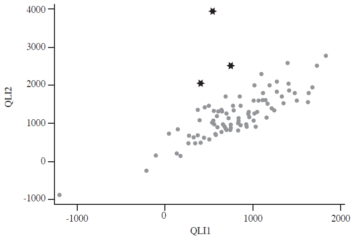
The advantage (or disadvantage) of the implicit prices methodology is that it may be used with different amenity bundles. Two different QLI were constructed to observe the consistency of the QLI itself when the amenities bundle changes. The first QLI1 includes only local taxes and the second QLI2 includes additionally local public investment in infrastructure. There are substantial differences in tax collection and grants allocation among cities in Mexico, which may affect how households may value external factors. For example, Mexico City collects an average of more than ten thousand pesos per household in taxes, but only receive little more than seven hundred pesos in local public infrastructure from federal grants. On the other hand, Nuevo Laredo collects almost nine hundred pesos in taxes per household but invests more than 14 thousand pesos in infrastructure using federal grants. The new valuation is, of course, product of the redistributive effect of grants. This fiscal allocation affects the valuation of the amenities bundle and the perception of quality of life. Something similar happened for other cities such as Cuernavaca and San Juan Del Río, who sharply improved in the ranking in similar manner. A scatter plot between QLI1 and QLI2, in figure 1, shows that for most cities the estimation of a QLI is fairly consistent as both QLIs are highly correlated¹⁰. The three cities that increase abruptly in the ranking due to unusually high level of federal grants are Nuevo Laredo, Cuernavaca and San Juan del Rio, marked with stars in Figure 1.

Figure 1: Correlation between two amenity bundles 

Another important consideration is the statistical confidence on the QLI ranking. We must be able to construct confidence intervals for each QLI in order to assess how much the position of a city may vary within the ranking. As we know, the amount of amenities in each city is fixed, at least in the period of analysis. Then, the only source of variability are the implicit prices. But in our theoretical setting, implicit prices are just weights obtained from a regression analysis on the overall sample. Therefore, we may use the standard deviation of each estimate to simulate implicit price variability.

We performed 1000 simulations on the implicit prices and recalculated the valuation of amenities for each city ¹¹. Then, we obtained the standard deviations for each QLI as shown in columns SD-1 and SD-2 in Table 5. With this information at hand, we are able to obtain confidence intervals to evaluate each city ranking. In the first ranking we observe that Campeche is still better than Acapulco at 95% confidence. But it is difficult to assess whether Veracruz is better than Villa de Alvarez as both are statistically similar and their confidence intervals overlap. There are similar cases where the QLI’s are very close to each other and differences in the ranking are not significant, some clear examples are Toluca and Monterrey or Chalco and Novojoa. The case of Oaxaca is noteworthy because is a city in the bottom of both rankings with a extremely low valuation.

Concluding remarks

Although the theoretical model is rather basic for our estimation, it offers powerful insights about the determinants of the spatial (non arbitrage) equilibrium among households and firms. The method of implicit prices offers a straightforward valuation of non-market goods and it is intrinsically linked to households’ welfare. In this sense, it is an objective method for estimation of non-market prices using information from visible market prices such as wages and rents. Implicit prices from Table 3 are weights (average) of such valuations for the whole group, in this case the Mexican households working in the private sector of the economy. They can be used for reference and also used for public policy design. Implicit prices in Table 3 tell us that public safety and access to basic education are highly valued within the Mexican Households’ utility. The third most valued amenity is the access to tertiary education (college and university). Then, any public policy designed to decrease crime rates and increase access and quality of basic and college education may certainly increase households’ welfare in Mexico. Coincidentally, in the present time, both public safety and basic education reform are the two top issues in the political agenda in Mexico.

The QLI is a construction that contains information of non-market prices but also about the mean provision of amenities (disamenities) in a specific location. It can also be tailored to match real-life preferences for certain amenities in any location, community, society or country. It offers the possibility to rank groups according to their valuation of these external attributes which allow us to design and target social and environmental policies. The QLI is not an all-purpose index, and it is only one of several analytical tools we may use to judge individuals’ well-being. The Bohemian Index, for example, is a different ranking of cities according to their urban infrastructure that foster a creative or bohemian class (high quality-highly developed human capital individuals). This index explains how cities enhance development according to their ability to attract creative individuals and subsequently, firms.

Our QLI ranking offers some interesting information on the valuation of amenities in different Mexican cities. With the present amenity bundles, it may be said that cities such as Campeche, Acapulco or Xalapa Enríquez have a high QLI and cities such as Oaxaca, Ciudad Cuauhtémoc and Ciudad Acuña have a low QLI. One important observation is that this ranking may be affected by the confidence interval of the explanatory variables. If the standard deviations of the estimates are large enough, it might be difficult to assert whether Campeche is absolutely better than Acapulco or if Oaxaca is absolutely worse than Ciudad Acuña, but it would be plausible that Campeche has a QLI higher than Oaxaca. This problem is particularly troublesome in the middle of the ranking. The confidence interval of the estimates might be affected by the statistical method used¹², but a straightforward use for a QLI might be just to compare cities in the very top of the ranking with those in the very bottom.

The two rankings of Table 5 give us important information on which Mexican cities the amenity bundles are more valued. The QLI cannot tell us whether an average household in Campeche is better off than an average household in Oaxaca. It rather tells us that the amenity bundle is more valued in Campeche than in Oaxaca by an average household. It would be difficult to affirm that changes in the ranking are exclusively due to changes in preferences alone. The QLI may be affected by the amenity package in some regions that might be determined by nature over time. Then, the QLI may change not only by the components in the bundle but also by changes on nature.

Another important consideration is the demographic changes (household structure). For example, young workers may prefer some cities while senior workers and retirees may prefer others, affecting indirectly implicit prices in such places. Furthermore, land supply and availability may be also restricted by institutional arrangements and geographical factors. Despite all these shortcomings, the QLI is still a valuable source of information to observe how some amenities (disamenities) influence household’s locational decision across Mexican cities.

Changes in the top of the ranking of Table 5 are more visible when federal transfers (grants) are included in the amenity bundle as a proxy of local public infrastructure. But some cities still remain in the top 20 and might be considered places with high quality of life, such as Acapulco or Campeche. But city ranking in the bottom remains almost unchanged even after the inclusion of transfers. The city of Oaxaca is of particular interest because it is in the bottom of both rankings with the highest crime rate, very little taxes and small investment in infrastructure.

Although there is no spatial analysis in this work, it might be noted that most cities close to the US border usually have a low QLI such as Ciudad Juarez, Mexicali and Tijuana though cities such as Heroica Matamoros are better ranked. The city of Nuevo Laredo became the first place in the second ranking when local public infrastructure is included. One possible interpretation for the case of Nuevo Laredo might be the federal and state grants for improvements in public safety, because border cities are relatively more exposed to criminal activity.

Cities within states along the Gulf of Mexico usually have high QLI. These cities have the advantage of low transport cost and access to better communication routes, though there are cities along the pacific coast that also have high QLI such as Acapulco, Tepic and Colima. Mexico City is a place where QLI is relatively low even though criminality is not a decisive issue compared with other cities with higher crime rate per cápita. The main disadvantage for Mexico City comes from the fiscal arrangements in place, where Mexico City residents are compelled to pay high taxes but receive relatively little transfers per cápita.

The QLI is a fairly good measure of the households’ valuation of amenities using information from households’ wage income and housing expenditure. In Mexico, it shows clearly that criminality is a bad and households are willing to pay for suppressing this disamenity. The QLI in this work may also be used as an instrument for public policy and can help to understand how Mexican households value their environment and are willing to pay for additional quantities of some amenities such as quality education.

The information from Table 5 offers important insights and can also be used for policy design. For example, investing in public safety and education in the bottom 10 cities in the ranking may not change significantly the ranking, but may reduce the relative distance between the low and high QLI cities. It is assumed that any change in the amenity bundle may affect the locational equilibrium, but we know that market prices may also adjust and, in this case, wages and housing prices will move to account for that change. So, there is no reason to expect many households relocating as many other conditions are fixed by nature (weather, coastal location, metropolitan areas, etc.). But as some other amenities such as the quality of education and public safety can be influenced directly or indirectly by policy, then the information in this work is certainly relevant for policy planners.

This work does not include the valuation of firms, and an extended model is needed to capture productivity differences among cities. This paper only offers information on the households’ side, and we must account for other complex factors that affect wages such as work effort or unionisation. Further research must be done to improve the theoretical framework and estimation methods on implicit prices that suit the Mexican spatial, demographic, social and economic reality.