


 nueva página del texto (beta)
 Inglés (pdf)
 Artículo en XML
 Referencias del artículo
 Enviar artículo por email
 Citado por SciELO
  Similares en
SciELO
Similares en
SciELO 
 Permalink
Introduction
In recent decades, due to a series of factors including demographic and cultural changes, an opening of its economy, a rise in the levels of formal education, the implementation of structural reforms which restructured the country’s economy towards a more service oriented one, and a series of crises that pushed women into the labour force, among others, female participation rates in Mexico have substantially increased.
According to information from Mexico’s population censuses, the percentage of women between 18 and 65 years of age participating in the labour force grew from 19.4% in 1970, to 24.2% in 1990 and to 42.3% in 2010. Consequently, analysis of the gender wage gap have become increasingly important, where a large number of studies have examined the evolution of male-female wage differentials in Mexico (e.g. Alarcón and McKinley, 1994; Pagán and Ullibarri, 2000; Popli, 2013). The rise in female labour participation rates has been accompanied by constant changes in the country’s occupational structure and distribution of wages between occupations (see, e.g. Brown, Pagán and Rodríguez-Oreggia, 1999; Rendón, 2003; Calónico and Ñopo, 2009). The present study attempts to examine these phenomena and contribute to the literature by examining the role of occupational segregation in explaining the gender wage gap in Mexico.4 An understanding of the factors driving male-female wage differentials is relevant since it helps direct public policies and evaluate if previous efforts to reduce gender wage inequalities have been rewarded.
The majority of studies that have examined gender wage differentials in Mexico have done so under the framework developed by Oaxaca (1973) and Blinder (1973), focusing on the issue of wage discrimination or unequal pay for equal work. Commonly referred to as the “index number” methodology, under Oaxaca-Blinder (OB) type decompositions, the discrimination effect is calculated as the unexplained difference between two reduced-form wage equations estimated separately for men and women. The estimation of these two wage equations is normally performed controlling for a standard set of productivity related variables, including variables denoting the individual’s occupational level, with the purpose of separating the effects of discrimination from those of legitimate compensating differentials (Reilly, 1991: 1). While including occupational controls allows interpreting the effect of the different occupational distributions of men and women, doing so is problematic since it assumes that occupations are exogenously given. Consequently, if occupational determination is subject to labour market discrimination, then this approach would be inappropriate (Liu et al., 2004).
Since the OB approach does not properly separate the effects of wage and job discrimination from those of occupational segregation, Brown, Moon and Zoloth (1980) suggest an alternative methodology that treats occupational choice as endogenously determined, and allows a decomposition of the wage gap into within and between occupational components.5 Under the Brown, Moon and Zoloth (BMZ) framework, the within and between components can be further decomposed into effects attributable to differences in observable characteristics and to differences in the estimated coefficients. In the context of between occupational effects, differences in the estimated coefficients provide an explicit estimation of the effect of occupational segregation on the gender wage gap. Identifying the relative importance of between against within occupational effects is important from a policy perspective, since the results may shed light on whether policies directed more at promoting equal pay within occupations should be prioritised, instead of measures that encourage a more equal access to different occupations (Liu et al., 2004).6
The present study contributes to the literature in several ways. First, an updated analysis based on the BMZ decomposition for the 2000-2010 period is performed. Furthermore, the Duncan and Duncan (1955) index of dissimilarity is also presented in order to provide an objective measure of the degree to which the occupational structures of males and females differ. Second, unlike previous studies that have emphasised the role of occupational segregation, we use census information which allows us to include rural localities and therefore study the entire Mexican labour market. Following Kidd and Shannon (1996) who raise awareness concerning the use of broadly defined occupational categories when performing wage decompositions, the much larger sample size of the census enables us to analyse the sensitivity of the results to the use of different levels of occupational aggregation. Third, in addition to the point estimates, we present standard errors for the different components of the Brown et al. (1980) decomposition. Finally, the sensitivity of the results is analysed where the estimated wage equations are corrected for self-selection into each occupation using the methodology outlined by Lee (1983).
Among the main results it is observed that gender wage differentials increased between 2000 and 2010. For both years, within occupation differentials positively contributed to the gender wage gap, whereas between occupation differentials provided a negative effect. Since within occupation differentials are driven by the unexplained component, the results suggest that the gender wage gap is primarily a product of differences in the average returns to productivity related characteristics within occupations. Furthermore, occupational segregation does not increase the gender wage gap since women do not appear to encounter barriers into high paying occupations. This result is robust to the use of different levels of occupational aggregation and when correcting the wage equations for selectivity-bias.
The study proceeds as follows. Section 2 presents a review of the related literature. Section 3 outlines the empirical and econometric methodologies. Section 4 describes the data and presents descriptive statistics. Section 5 discusses the main results. Section 6 tests the sensitivity of the results. Section 7 concludes.
Literature review
The literature that has examined gender wage differentials in Mexico is extensive. These studies usually report that women earn less than men, where the magnitude of the gender wage gap fluctuates depending on the period of study and the geographical coverage of the data source used.
Among the studies that have used the OB framework to examine gender wage differentials, Alarcón and McKinley (1994), based on data from the Encuesta Nacional de Ingresos y Gastos de los Hogares (ENIGH, National Household Income and Expenditure Survey) from 1984, 1989 and 1992, observe that the gender wage gap increased from 23.3% in 1984, to 28.4% in 1989 and to 25.3% in 1992. In addition, for all three periods, the scholars find that at least 70.0% of the wage gap is attributed to discrimination, i.e. to differences in the economic returns to average characteristics.7 Based on data from the ENIGH from 2000, Martínez and Acevedo (2004) observe that approximately 85.0% of the gender wage gap is a product of differences in the economic returns to average characteristics. Alternatively, Mendoza and García (2009), using data from the Encuesta Nacional de Ocupación y Empleo (ENOE, National Occupation and Employment Survey) from 2006, observe that the majority of the gender wage gap, i.e. 87.6%, is a product of differences in average characteristics. Moreover, the authors report that this figure varies significantly by region, where gender wage discrimination is smallest in the north of Mexico and largest in the south.
Using an alternate methodology, Pagán and Ullibarri (2000), based on data from the Encuesta Nacional de Empleo Urbano (ENEU, National Urban Employment Survey) from 1995, analyse the role of group heterogeneity, i.e. differences by education level, age, firm size, sector of employment, and region of residence, on the gender earnings gap. The authors compute selectivity corrected earnings equations and estimate an additively decomposable index of the extent of gender unexplained wage inequality based on Jenkins (1994). The study shows that the unexplained wage gap is larger among workers with high education levels, which have full-time jobs, work in micro-firms, and are employed in the informal sector. On the other hand, Pagán and Sánchez (2000) use the Encuesta Regional de Servicios Financieros a Unidades de Protección Rural (SREFS, Survey of Rural Entrepreneurs and Financial Services) to study the factors that explain gender differences in workforce participation and in the incidence of self-employment in rural Mexico. Estimating a bivariate probit to analyse the propensity of individuals to enter the workforce and examine the incidence of self-employment among the employed, the authors show that if the female employment rate is predicted under the assumption that women face the male labour market structure, gender employment rate differentials almost disappear. While 88.2% of gender employment rate differences can be explained by structural demand and supply factors, only 11.8% is attributable to differences in individual endowments. Although the authors do not explicitly explore gender wage differentials, the results suggest that gender-related labour market discrimination is likely to be present in the wage or salaried sector.
Studies that emphasise the role of occupations when examining the gender wage gap in Mexico include Sánchez (1998), where the author employs the BMZ decomposition to evaluate the impact of between and within sectoral factors on male-female earnings differentials among rural and urban microenterprises. Based on data from the SREFS from 1994 and the Encuesta Nacional de Micronegocios (National Survey of Urban Microenterprises) from 1992, it is observed that female-headed microenterprises in rural and urban areas earn 64.0% and 50.0% less, respectively, than male-headed microenterprises. In addition, an estimated 35.0% of the earnings gap in urban areas can be attributed to differences in average characteristics, whereas in rural areas this figure rises to 42.0%. Only a small share of the gender earnings gap is explained by differences in sectoral distributions. In a descriptive analysis, Rendón (2003) examines gender differences in employment, segregation and wages. Based on various data sources including the 1990 and 2000 Population Censuses and the Encuesta Nacional de Empleo (ENE, National Employment Survey) from 2000, the author reports that male hourly wages surpass those of females by approximately 9.0%, where this gap varies significantly depending on the sector of employment. In addition, the scholar reports that women tend to be concentrated in specific occupations. When analysing the sector of employment of women, an increase in segregation by production sector between 1990 and 2010 is observed. Moreover, the study reports that there is high degree of vertical segregation in the Mexican labour market, where men tend to occupy higher ranking and better paying positions than women.8
Using data from the ENEU, Brown et al. (1999) examine the effect of occupational attainment on the increase in the gender wage gap between 1987 and 1993. The study uses the Wellington (1993) decomposition to disaggregate wage gap changes into relative changes in personal characteristics and changes in the returns to these characteristics. The authors also decompose gender differences in earnings between occupations and analyse the role of occupational attainment in the overall earnings gap by using the BMZ methodology. The results show that during the period of study there was an increase in the gender earnings gap attributed to relative changes in human capital endowments since, all else equal, wage coefficient changes would have slightly reduced the gender earnings gap. Moreover, while in 1987 the explained component accounted for 68.0% of the earnings gap, in 1993 it represented close to 73.0%. Furthermore, the gender earnings gap was mitigated by a substantial decline in gender differences in occupational attainment. The scholars also use the OB decomposition to study the effects of the occupational structure on the wage gap. It is observed that the majority of the earnings gap is a product of unexplained differences. When occupational controls are included, the authors find that occupational segregation reduces earnings differentials. In another study, Calónico and Ñopo (2009), based on data from the ENEU from 1994 to 2004, use a matching comparisons technique to examine the role of individual and family characteristics in determining gender segregation and wage gaps. The scholars report that the elimination of vertical segregation would decrease the gender wage gap by 5.0 percentage points. On the other hand, the elimination of occupational segregation would increase gender wage differentials by 6.0 percentage points. Furthermore, it is observed that, during the period of study, the role of occupational segregation in determining the gender wage gap increased, whereas the relative importance of vertical segregation decreased.
Recent studies have focused on studying the gender wage gap at different parts of the wage distribution. Among these, using primarily census data from 1990 to 2010, employing the methodology put forward by DiNardo, Fortin and Lemieux (1996) and correcting the analysis for selection of women into the labour market, Campos-Vázquez and Arceo-Gómez (2014) observe a consistent pattern of “sticky floors” and a decreasing pattern of “glass ceilings” over the period of study. In addition, the authors report that the majority of the gender wage gap is a result of differences in prices. Moreover, the scholars show that the gender wage gap becomes larger when correcting for selection, which suggests that women are positively selected into the labour market. Finally, Popli (2013) also examines gender wage differentials throughout the entire distribution in both the formal and informal sectors based on data from the ENIGH from 1996 and 2006. Taking into account the probability of employment into the wage or salaried sector, the study finds that the gender wage gap differs considerably by sector of employment. Contrary to raw gender wage differentials, the selection-adjusted gender wage gap is higher in the formal sector compared to the informal sector. Using different techniques including the OB decomposition, the measure proposed by Jenkins (1994) and non-parametric techniques, the scholar shows that the unexplained gender wage gap varies according to the sector of employment, where the unexplained term is higher in the formal sector relative to the informal sector. The study also reports that in both sectors the unexplained gender wage gap decreased during the period of analysis, where there is evidence of a “glass ceiling” in the formal sector, with the unexplained male-female wage gap being higher in the upper tail of the distribution.
Methodology
The decomposition developed by Brown et al. (1980), i.e. the BMZ decomposition, requires the estimation of occupation-specific wage regressions for male (m) and female (f) workers:
where w
ik
represents the natural logarithm of hourly wages for individual i employed in occupation
where adding and subtracting terms on the right hand side of Eq. (3) and manipulating terms yields Eq. (4). In the decomposition,
In addition to the occupation specific wage regressions, the BMZ decomposition requires a method for predicting
where
To obtain
Data description
The data used in this study comes from a 10.6% and 10.0% random sample of Mexico’s 2000 and 2010 Census of Population and Housing, respectively. The information is collected by the Instituto Nacional de Geografía y Estadística (INEGI, National Institute of Geography and Statistics) and provided by IPUMS-International (2013). The sample includes full-time salaried workers between the ages of 18 and 65 years that report non-zero wages.10 Furthermore, workers located at the bottom and top 0.5% of the wage distribution are omitted in order to eliminate the effects generated by the presence of outliers. All figures are in real June 2010 Mexican pesos (MXP).
Given its substantial sample size, the use of census data provides a clear advantage over Mexico’s traditional labour force surveys, i.e. the ENEU, ENE and ENOE. The census allows having a larger number of observations for each individual occupation and allows using a more disaggregated occupational classification scheme. The use of smaller samples has its drawbacks as it may lead to the use of more broadly defined occupational categories, which in turn may hide wage differences and heterogeneity within generally defined occupations.
Descriptive statistics
Table 1 presents descriptive statistics, where significant differences between male and female characteristics are observed. Among these, for both 2000 and 2010 mean log hourly wages of men are larger than those of women. Specifically, this figure is .021 log points higher in 2000 and .026 log points higher in 2010.11 A similar relationship is observed regarding the age structure, where in both periods men are slightly older than women. Given that age is positively correlated with labour market experience, this suggests that one of the reasons why male wages are higher is because on average they have more experience than their female counterparts. With respect to human capital levels, on average female workers have higher education levels than males. This difference slightly increased during the period of study, going from 1.34 years in 2000 to 1.36 years in 2010. The fact that women have higher levels of education but lower hourly wages than men implies that their returns to education may be smaller. On the other hand, men have substantially longer work-weeks than women and have a lower likelihood of engaging in part-time work. The difference in the size of the work-week is one of the main factors behind the observed gender wage gap when focusing on weekly wages. Moreover, for both 2000 and 2010, women have higher participation rates in the formal sector than men, which tends to be associated with higher productivity levels and therefore higher wages. In addition, male salaried workers have a higher probability of being married than their female counterparts. Since labour force participation rates differ substantial between male and female workers, this may be signalling that women are likely to drop out of the labour force once they engage in marriage. In summary, taking the above differences into consideration, it cannot be ruled out that the gender wage gap may be driven by socioeconomic and demographic characteristics instead of other factors such as occupational segregation.12
Table 1 Descriptive statistics, means and standard errors
| Variable | 2000 | 2010 | ||
|---|---|---|---|---|
| Men | Women | Men | Women | |
| Log hourly wages | 2.933 | 2.912 | 3.159 | 3.133 |
| (0.706) | (0.711) | (0.639) | (0.665) | |
| Age | 33.97 | 32.31 | 35.83 | 35.40 |
| (11.14) | (10.13) | (11.49) | (10.74) | |
| Schooling | 8.500 | 9.839 | 9.677 | 11.04 |
| (4.407) | (4.253) | (4.337) | (4.229) | |
| Hours worked per week | 45.35 | 43.35 | 45.48 | 43.59 |
| (6.085) | (6.514) | (6.115) | (6.497) | |
| Formal | 57.98 | 68.19 | 55.80 | 66.10 |
| Married | 72.50 | 43.51 | 71.59 | 48.18 |
| Rural | 17.44 | 8.118 | 17.18 | 8.705 |
| Part-time employment | 5.944 | 14.73 | 7.438 | 15.59 |
| Labour force participation | 88.73 | 36.95 | 90.85 | 43.00 |
| Unemployment rate | 1.479 | 0.894 | 5.591 | 2.734 |
| Observations | 780.987 | 362,879 | 794,462 | 379,410 |
Source: Authors elaboration based on the 2000 and 2010 Mexican Census. Data includes individuals between 18 and 65 years of age. Hourly wages are in natural logarithms and in real June 2010 MXP. Standard errors are in parentheses.
Turning our attention to mean log hourly wages within occupations, some interesting results emerge. As seen in Table 2, for both periods within all occupational categories men have higher wages than women. In the year 2000, the gender wage gap was the largest at the “Crafts and related trades workers” category, rising to .303 log points, and it was the smallest at the “Technicians and associate professionals” category, standing at .048 log points. At the highest paying occupation, i.e. the “Legislators, senior officials and managers” category, the male-female wage differential was also substantial, where it was equal to .210 log points. In 2010, the gender wage gap was the largest at the “Plant and machine operators and assemblers” category, rising to .277 log points, and it was the smallest at the “Skilled agricultural and fishery workers” category, standing at .004 log points. Finally, in 2010 at the top of the occupational distribution the male-female wage gap decreased to .083 log points.
Table 2 Log hourly wages by occupation, means and standard errors
| Occupation | 2000 | 2010 | ||
|---|---|---|---|---|
| Men | Women | Men | Women | |
| Legislators, senior officials and managers | 4.107 | 3.897 | 3.895 | 3.812 |
| (0.730) | (0.698) | (0.655) | (0.648) | |
| Professionals | 3.869 | 3.683 | 3.931 | 3.849 |
| (0.626) | (0.595) | (0.629) | (0.617) | |
| Technicians and associate professionals | 3.317 | 3.269 | 3.578 | 3.533 |
| (0.600) | (0.601) | (0.596) | (0.595) | |
| Clerks | 3.245 | 3.121 | 3.255 | 3.214 |
| (0.650) | (0.590) | (0.550) | (0.523) | |
| Crafts and related trades workers | 2.925 | 2.622 | 3.186 | 3.086 |
| (0.573) | (0.537) | (0.533) | (0.718) | |
| Service workers and shop and market sales | 2.902 | 2.642 | 3.071 | 2.874 |
| (0.631) | (0.628) | (0.590) | (0.561) | |
| Plant and machine operators and assemblers | 2.893 | 2.669 | 3.091 | 2.814 |
| (0.488) | (0.360) | (0.513) | (0.389) | |
| Elementary occupations | 2.647 | 2.425 | 2.833 | 2.751 |
| (0.491) | (0.519) | (0.463) | (0.464) | |
| Skilled agricultural and fishery workers | 2.271 | 2.139 | 2.613 | 2.609 |
| (0.539) | (0.557) | (0.493) | (0.484) | |
| Observations | 780,987 | 362,879 | 794,462 | 379,410 |
Source: Authors elaboration based on the 2000 and 2010 Mexican Census. Data includes individuals between 18 and 65 years of age that work 30 or more hours per week. Hourly wages are in natural logarithms and in real June 2010 MXP. Standard errors are in parentheses.
Results
The first-stage of the Brown et al. (1980) decomposition requires the estimation of K occupation specific wage regressions for male and female workers as defined in Eqs. (1) and (2), and a MNL occupational attainment model as defined in Eq. (5). While we do not present the first-stage estimations due to space constraints, we briefly discuss the main findings. Furthermore, these results are available upon request.
The estimation of nine occupation specific wage regressions show that there are significant differences in the returns to education between men and women. In 2000, in the “Legislators, senior officials and managers” category, males had higher returns to education than females. In the rest of the distribution, the returns to education of males and females were similar with the exception of the “Plant and machine operators and assemblers” category, where the returns for males were substantially larger. By 2010, female returns to education surpassed those of males in the top paying category and were similar among all workers in the rest of the occupational distribution. Based on the previous outcomes, it can be inferred that gender differences in returns to schooling are in large part driven by dissimilarities in the occupational structures. Regarding the returns to potential experience, in both 2000 and 2010, women were better compensated than men for low experience levels in the highest paying occupations. On the other hand, in the lower part of the occupational distribution, the returns to experience were larger for men. Additional results are as expected, where being in formal employment, married and working in an urban locality are positively related with higher hourly wages. Moreover, the state unemployment rate is negatively correlated with hourly wages, particularly in the highest paying categories. In summary, the results show that there is substantial variation in the effects of the covariates on male and female wages depending on the occupation of employment.
Attention now turns to the MNL occupational attainment model, where the “Elementary occupations” category was used as the reference group. Among the explanatory variables, education plays an important role in predicting employment into the two highest paying occupations, i.e. the “Legislators, senior officials and managers” and “Professionals” categories. The effect of education is strongest among women and is significant in both 2000 and 2010. A different story emerges in low skilled categories, where an additional year of schooling has either a much smaller effect or reduces the probability of attachment. Regarding potential experience, in 2000 this was generally associated with an increase in the probability of attachment at the top of the distribution. Moreover, its effect was larger among males and negative for females in low-paying categories. While a similar relationship is observed among males in 2010, for females experience it was positively associated with attachment in the highest-paying occupation and negatively associated with attachment in other occupations. On the other hand, variables related to the worker’s family situation show that, in 2000, the married population had a higher probability of being employed outside of the “Elementary occupations” category, where the size of this coefficient was fairly stable across occupations. In 2010, whereas a comparable relationship was observed among women, no clear pattern emerged among males. Pertaining to the number of children under age six, in the year 2000 this had a negative effect on the probability of working in the “Legislators, senior officials and managers” category for all workers, although the coefficients are not statistically significant. A different relationship is observed in 2010, where the coefficient was positive for both genders at the top of the occupational distribution, although it was only significant for women. Regarding family size, for both periods and genders, the variable had a negative effect on the probability of attachment in the highest paying occupations. Altogether, the effect of the explanatory variables on occupational attainment varies according to the gender and between periods. This suggests that men and women are allocated differently between occupations based on their observed characteristics.
Brown-Moon-Zoloth decomposition
The results of the BMZ decomposition of log wage differentials between men and women disaggregated by year and locality size are presented in Table 3. In 2000, the hourly log wage differential between men and women stood at .021 log points. The sum of the WE and BE components, which equalled -.043 log points, suggests that according to their average characteristics women actually should have had higher hourly wages than men. Nonetheless, analysing these two terms separately shows substantial heterogeneity in their effects. Specifically, the WE component, which rose to .023 log points, was roughly equal to the total gender wage gap. This implies that the entirety of the gender wage gap was accounted for by differences in average characteristics. On the other hand, the BE component stood at -.066 log points indicating that, on average, women were allocated in better remunerated positions than men. With respect to the unexplained components which capture differences in coefficients, the sum of the WU and BU terms was equal to .064 log points or 304.7% of the gender wage gap. This signals that based on the returns to their average characteristics, the size of the gender wage gap should have been larger than what is in fact observed. Nonetheless, when separating the two unexplained components significantly different patterns emerge. The WU term, equivalent to .167 log points, suggests that wage differentials are largely driven by vertical segregation, i.e. by differences in the returns to average characteristics within each occupation. On the other hand, the BU component which captures the effect of occupational segregation negatively contributes to the gender wage gap. Somewhat surprisingly, this implies that women encountered fewer barriers to entry into high paying occupations than men.
Table 3 BMZ decomposition of log hourly wage differentials between men and women
| 2000 | 2010 | |||||
|---|---|---|---|---|---|---|
| Total | Urban | Rural | Total | Urban | Rural | |
| Total log hourly wage differential | .021 | .081 | .017 | .026 | .066 | .007 |
| (.001) | (.001) | (.002) | (.001) | (.001) | (.002) | |
| Explained: Differences in mean characteristics | ||||||
| Within | .023 | .026 | .009 | -.018 | -.017 | -.007 |
| (.001) | (.001) | (.001) | (.001) | (.001) | (.001) | |
| Between | -.066 | -.046 | -.103 | -.030 | -.025 | -.075 |
| (.001) | (.001) | (.001) | (.001) | (.001) | (.001) | |
| Unexplained: Differences in coefficients | ||||||
| Within | .167 | .165 | .209 | .132 | .134 | .152 |
| (.001) | (.001) | (.002) | (.001) | (.001) | (.002) | |
| Between | -.103 | -.064 | -.098 | -.058 | -.026 | -.063 |
| (.001) | (.001) | (.002) | (.001) | (.001) | (.002) | |
Note: Male OLS coefficients are taken as the non-discriminatory vector.
Source: Authors elaboration based on the 2000 and 2010 Mexican Census. Standard errors are in parentheses. Decomposition based on OLS regressions which include as independent variables years of education, potential experience, potential experience squared, the state unemployment rate, and dummy variables for marital status, formal-informal work and region of residence.
With respect to differences between urban and rural localities, the gender wage gap varies significantly when making this distinction, rising to .081 and .017 log points in urban and rural settings, respectively. In addition, in urban localities the sum of the WE and BE components equalled -.020 log points. On the other hand, in rural areas the WU and BU components totalled .101 log points.
In 2010, the gender wage gap stood at .026 log points. With the exception of the WE term which equalled -.018 log points, the sign and overall interpretation of the different components of the BMZ decomposition are generally similar to those observed in 2000. The negative sign of the WE component suggests that according to their average characteristics within occupations, female hourly wages should have been higher than those of males. Moreover, the BE component which stood at -.030 log points denotes that, on average, women were allocated in better remunerated positions than men. Relative to 2000, the reduction in absolute value of the BE term signals that, while in 2010 women still occupied better compensated positions than men, male-female occupational structures became more alike during this period. Concerning the unexplained components, the sum of the WU and BU terms totalled .074 log points or 284.6% of the wage gap. While the WU component stood at .132 log points, its reduction with respect to 2000 implies that the differences in the returns to average characteristics between men and women decreased by 21.0% during the period of study. The decline in the WU term between 2000 and 2010 signals a positive change towards a more equal wage compensation within occupations among men and women. On the other hand, the contribution of occupational segregation to the wage gap captured through the BU component was again negative, although smaller in absolute value relative to 2000. This suggests that in 2010, women still encountered fewer barriers to entry into high paying occupations than men. Moreover, the statistically significant effect of the BU term in 2000 and 2010 implies that, in both periods, workers were assigned to different occupations based on non-productivity related characteristics.
Finally, gender wage differentials once again differ when making the distinction according to the size of the locality of residence. Specifically, the wage gap stood at .066 and .007 log points in urban and rural localities, respectively. In urban areas, the sum of the WE and BE terms equalled -.042 log points, while in rural localities the sum of the WU and BU components totalled .089 log points.
Differences in the occupational structure
The observed and predicted occupational distributions of men and women across the nine occupational categories for 2000 and 2010 are presented in Table 4, where the allocation rule of males, derived from Eq. (5), is used to obtain the female simulated occupational structure. This scenario can be interpreted as men and women having similar preferences and the labour market providing equal opportunity and occupational access to both groups. Furthermore, the Duncan and Duncan (1955) index of dissimilarity is used in order to provide a better understanding of the degree of gender differences in the occupational structures. The index is given by:
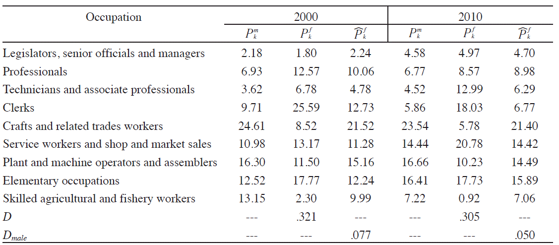
Source: Authors elaboration based on the 2000 and 2010 Mexican Census. Predicted distribution by occupation represents the proportion of female workers who would be in each occupation if they were to follow the same occupational sorting function as men, based on the estimation of a MNL model of occupational attainment for male workers.
Table 4 Distribution by occupation and dissimilarity indices
where Eq. (6) is interpreted as measuring the proportion of male workers required to change occupations in order to obtain the same occupational distribution generated by female workers. An index value equal to zero reflects that there is no occupational dissimilarity between both groups. On the other hand, an index value equal to one indicates that men and women are never in the same occupations.
With respect to the observed occupational distribution, in 2000, at the extremes of the distribution, men had higher participation rates in both the highest paying occupation, i.e. in the “Legislators, senior officials and managers” category, and in the lowest paying one, i.e. in the “Skilled agricultural and fishery workers” category. Nonetheless, at the middle of the occupational distribution, a different picture emerges. In general, women had higher participation rates than men at the top-half of the distribution, whereas at the bottom-half no clear pattern is observed. Focusing on the Duncan index of dissimilarity, it shows that, in 2000, approximately 32.1% of women would have needed to change occupations in order to obtain the same occupational distribution as men. On the other hand, in 2010, women had higher participation rates than men in the four highest paying occupations. Furthermore, while the share of female workers employed in the “Elementary occupations” category remained relatively stable between 2000 and 2010, a much larger proportion of men were employed in this category at the end of this period. As a result, the Duncan index slightly decreased to .305 in 2010.
Comparing observed distributions to predicted ones, according to the male allocation rule, female workers were under-represented at the “Legislators, senior officials and managers” category in 2000, but not in 2010. In both 2000 and 2010, women were under-represented at the bottom of the occupational distribution. This result can be inferred since under the male occupational sorting function female workers had a much larger participation rate in the “Skilled agricultural and fishery workers” category compared to their actual share. On the other hand, in both years, women were over-represented in the “Elementary occupations” category, which is one of the lowest paying occupations and employs a much larger share of male and female workers.
When women follow the same allocation rule as men, the Duncan index is reduced significantly to 7.7% in 2000 and 5.0% in 2010. Jointly, the previous findings imply that only a small part of the differences in the occupational structures between men and women are driven by different sorting functions. These dissimilarities are likely a product of differences in productivity related characteristics and cultural factors which assign different roles in the labour market for men and women.
Sensitivity checks
Different levels of occupational aggregation
Because of computational problems and the presence of small cell sizes within certain occupations, the majority of studies that employ the BMZ decomposition use a very aggregated level of occupational classification.13 Nevertheless, the use of broadly defined categories conceals the importance of occupations when performing wage decompositions, since it likely conceals significant wage differences and heterogeneity within the generally defined occupations. To examine the sensitivity of our results to the number of categories, the analysis is performed under different levels of occupational aggregation.
The results of the BMZ decomposition at the one-digit and two-digit occupational aggregation levels are presented in Table 5.14 For 2000, augmenting the number of categories did not increase the proportion of the wage gap attributed to the explained component, i.e. the sum of the WE and BE terms. On the contrary, it decreased from -.043 log points at the one-digit level to -.052 at the two-digit level. Moreover, the WE, BE and WU components were marginally reduced, while the BU term was subject to an increase. For 2010, expanding the number of categories led to a slight increase in the proportion of the wage gap attributed to the explained component, where the sum of the WE and BE terms rose from -.048 log points at the one-digit level to -.036 log points at the two-digit level. Moreover, while the WE component grew by .019 log points, the BE term was reduced by .007 log points.
Table 5 Sensitivity of BMZ decomposition of log hourly wage differentials between men and women to different levels of occupational aggregation
| Number of occupations | 2000 | 2010 | ||||||
|---|---|---|---|---|---|---|---|---|
| WE | BE | WU | BU | WE | BE | WU | BU | |
| One-digit | .023 - | .066 | .167 | -.103 | -.018 | -.030 | .132 | -.058 |
| (.001) | (.001) | (.001) | (.001) | (.001) | (.001) | (.001) | (.001) | |
| Two-digit | .016 | -.068 | .150 | -.078 | .001 | -.037 | .123 | -.062 |
| (.001) | (.001) | (.002) | (.001) | (.001) | (.001) | (.002) | (.001) | |
Note: One-digit denotes nine occupational categories for 2000 and 2010. Two-digit denotes 18 occupational categories for 2000 and 49 categories for 2010.
Source: Authors elaboration based on the 2000 and 2010 Mexican Census. Standard errors are in parentheses.
In general, the main results for the year 2000 are not very sensitive to the number of categories, since augmenting the number of occupations does not increase the proportion of the gender wage gap attributed to the explained component. On the other hand, for 2010 the WE term varies considerably between the one and two-digit levels, suggesting that this component is sensitive to the number of occupational categories. Nonetheless, the fact that the BU term is always negative and remains relatively stable provides further evidence that occupational segregation does not increase the gender wage gap in Mexico.
Controlling for self-selection
Since occupational attainment is determined by the interaction between demand and supply factors where individuals may differ among unobservable characteristics between occupations, the sample of workers observed in each occupation may not be random. In this section, we use the information obtained from Eq. (5) to adjust the occupation specific wage equations for potential effects generated by selection bias. Following Lee (1983), the wage equations are modified accordingly and conditional on occupation k being chosen are given by:
where
In Eq. (7),Φ is the standard normal probability density function, σ k is the standard error of the disturbance term, and ρ k is the correlation between the error terms of Eqs. (5) and (7). The function is a strictly increasing transformation that converts the random variables associated with occupational attainment into a standard normal variant, i.e. τ=Φ -1- (F), where Φ is the standard normal cumulative distribution function, and F is the distribution function of the MNL as defined in Eq. (5).
The procedure is carried out in two stages. First, estimates of the coefficient vector in the MNL equation are obtained from Eq. (5). Second, these estimated coefficients are used to calculate λ ik . The variables included in the vector Z ik are expected to affect the worker’s desire for a particular occupation as well as the willingness of employers to hire the individual. The analysis uses as excluded instruments that identify selectivity indicators for the number of children below six and household size. It is assumed that these demographic variables shift the probability of being employed in occupation k but do not affect wages. Nonetheless, attaining identification in the selectivity model is challenging given that no available variable can be considered a completely exogenous instrument.
The results of the BMZ methodology controlling for self-selection into occupations are presented in Table 6.15 In these estimations, the correction term is not considered as constituting part of the explained or unexplained components and instead is examined separately. Moreover, the four previously defined terms of the decomposition are grouped and demarcated as representing the wage offer gap or unconditional wage differential. This is equivalent to setting the selectivity effects to zero in each equation, where the wage offer gap is taken to indicate the wage a worker randomly drawn from the population would receive if she or he were selected into the occupational category in question (Gyourko and Tracy, 1988).
Table 6 BMZ decomposition of log hourly wage differentials between men and women with Lee (1983) correction
Note: Male OLS coefficients are taken as the non-discriminatory vector.
Source: Authors elaboration based on the 2000 and 2010 Mexican Census. Standard errors are in parentheses. Decomposition based on OLS regressions which include as independent variables years of education, potential experience, potential experience squared, the state unemployment rate, a selection term, and dummy variables for marital status, formal-informal work and region of residence.
Among the results, it can be seen that the selection term differential is always positive, implying that the wage offer gap is smaller than the total wage gap, and that gender wage differentials are smaller and negative after correcting for self-selection. Moreover, for the full sample in both 2000 and 2010, the BE term now stands at -.085 and -.057 log points, respectively. This reinforces the result obtained in Section 4 which indicates that, on average, women are allocated in better remunerated positions than men. A similar finding is observed when dividing the sample between urban and rural workers. On the other hand, when controlling for self-selection the WU term is no longer the main driver of the gender wage gap, since this component is now considerably smaller for both years and across different samples. Instead, the gender wage gap is mostly a product of differences in the selection term. Furthermore, there are considerable differences in the magnitude of the WU across time, where this component stood at .002 and -.075 log points in 2000 and 2010, respectively. These results suggest that when controlling for self-selection, women do not appear to encounter vertical or hierarchical segregation in the labour market. Regarding the BU component, it is once again observed for the full sample in 2000 and 2010 that this term negatively contributed to the total wage gap. This implies that women encountered fewer barriers to entry into high paying occupations than men, where the effect of the BU term is now bigger in absolute value. Additionally, the WE term went from positively contributing to the gender wage gap in 2000 to having a negative effect in 2010. Moreover, the BE component increased from -.085 to -.057 log points, whereas the BU term increased from -.130 to -.085 log points.16
Conclusions
This study examined the role of occupational segregation in explaining the gender wage gap in Mexico. Based on the BMZ decomposition, the results show that male-female hourly wage differentials increased between 2000 and 2010. For both years, the sum of the within occupation wage differentials components positively contributed to the total gender wage gap, whereas the sum of the between occupation wage differentials components had the opposite effect. The gender wage gap is mostly a product of compensating differences within rather than across occupational categories. Furthermore, since within occupation wage differentials are largely driven by the unexplained component, the findings suggest that the gender wage gap is primarily a product of differences in the average returns to productivity related characteristics within occupations. While the study shows that the occupational structure of male workers differs considerably from that of their female counterparts, occupational segregation does not increase the gender wage gap, since women do not appear to encounter barriers into high paying occupations. The effect of the role of occupational segregation is robust to the use of different levels of occupational aggregation and remains relatively stable when correcting the occupation-specific wage equations for selectivity-bias using the methodology outlined by Lee (1983).
While occupational segregation does not play an important role in the wage disadvantage experienced by women, it is likely that the gender wage gap is mostly driven by partial segregation within the defined occupational categories given the large values of the within unexplained component. Consequently, the implementation of policies intended at balancing gender representation across occupations can have only a limited effect and are likely to be less effective than policies designed at undoing partially segregated positions within given occupations. Future legislation should be directed at encouraging equal pay within occupations rather than at endorsing a more equal distribution of men and women across occupations. Moreover, the fact that senior positions tend to be occupied by males while the subordinates are commonly female is likely to represent an ineffective allocation of human resources which generates inefficiencies in the labour market.

