


 text new page (beta)
 English (pdf)
 Article in xml format
 Article references
 Send this article by e-mail
 Cited by SciELO
  Similars in
SciELO
Similars in
SciELO 
 Permalink
Introduction
Many developing countries seem to be undergoing various structural transformations towards to achieve sustainable economic development. The importance of health status, human capital or pollution levels have been increasing in these countries. During the past couple of decades as a developing country, Turkey has also been going through a transformation process from agrarian to industrialization. Turkey has achieved to have an astonishing economic performance after the large scale economic crisis in 2001. Especially during the period of 2002 and 2007, there exists a high level of growth. After the world crisis in 2008, the growth rate of Turkey is declined. It is assumed that economic growth brings improvement in the inequality. The distributional effects of growth on different income groups may cause deterioration in some developing economies. During that period, the income inequality of Turkish economy does not improve as it is expected (see Figure 1).

Source: Own elaboration.
Figure 1 Gini coefficients of OECD countries for the late-2000s. (OECD ,2011)
There could be some adverse distributional impacts of economic growth on the income distribution.2 During the economic growth and development process, income inequality worsens for specific income groups. In the absence of appropriate level of environmental regulation, industrialization and urbanization leads to deterioration of air quality, and this in turn undermines health. According to some studies in the literature,3 low-income groups are affected more from air pollution compared to high-income groups. Actually, this effect comes from the fact that the former has lower health status due to lack of environmental precautions. Individuals in this group may presumably be exposed more to environmental pollutants. Although income inequality is an important component for the health status, the link between income inequality and air pollution is missing in a widespread manner.
The literature on the relationship between income inequality and health; air pollution and health; and finally, income inequality and air pollution are enormous. Following Rodgers (1979) who reveals that inequality has an impact on health status both in developed and developing countries, Wilkonson (1992) examines whether inequality is a crucial determinant of health status for specific developed countries. Besides the country level investigations, some of the studies investigate the effect of inequality on pollution at different region-levels such as states, metropolitan areas (Blakely et al., 2002; Lopez, 2004; Subramanian et al., 2001). Subramanian and Kawachi (2004) summarize the literature on the effect of inequality on health for the US. They show comparative results of different studies which all stress the negative impact of inequality on health. Although, majority of the studies in the literature agree with the negative impact of inequality on health, some reject this finding (Deaton, 2003; Mellor and Milyo, 2001; Wilkinson and Pickett, 2006). A recent study (Feng et al., 2012) explores the effects of income inequality on health outcomes of the elderly using multilevel logistic models.
The effect of air pollution on the health status is examined in many studies (Luginaah et al., 2002; Wilson et al., 2004). Some of them focus on the relationship of morbidity and mortality to air pollution. These studies reveal that the exposure to gradually increasing air pollution raises morbidity and mortality (Pope et al., 2002; Krewski et al., 2000; Zanobetti et al., 2000; Pope and Dockery, 1999). Hansen and Selte (1997) are concerned with to which extent health effects in turn induce sick-leaves (a reduced labor productivity) as a cost of air pollution and employed multinomial logit model to analyze this linkage.
There is also a large literature on the link between income inequality and air pollution, which is also our primary interest in this work, Charafeddine and Boden (2008) argue that individuals in regions with higher income inequality are exposed to higher level of air pollution compared to those individuals living in more equal regions and they use a multilevel (hierarchical) logistic regression to model the association between general self-reported health and fine particulate pollution accounting for income inequality. Additionally. Torras and Boyce (1998) reveal the relationship between US state-level income inequality and state-level environmental stress, showing that the higher the inequality the higher is the stress. It is straightforward that higher inequality may increase the crime level and violence and so may the stress. This is discussed in Kawachi et al., (1999); Wright and Steinbach, (2001).
Although empirical results are far from consensus, many theoretical studies describe mechanisms for the negative impact of income inequality on health via air pollution. This paper will contribute to empirical literature by studying the Turkish case. In fact, given the level of air pollution and income inequality problems (although the inequality has been improved over the last decade) in Turkey, relatively little attention has been paid on this problem. The main objective of this paper is to investigate the importance of income inequality on the link between air pollution and health. For the empirical analysis, we obtained the required data from the Survey of Income and Living Conditions (SILC) conducted by the Turkish Statistical Institute (TurkStat) for the years 2009 and 2010 for socio-economic and health related variables. Air pollution data is drawn from TurkStat’s Air Quality Statistics data. We use nested and multinomial logistic regression analysis to examine the effects of air pollution and income inequality on health status.
The present paper is organized as follows. In the next section we provide data, the methodology. In section 3 we make the empirical analysis. Finally, Section 4 focuses on some concluding remarks and discussion.
Data and methodology
Data
For this research, we use the Survey of Income and Living Conditions (SILC) conducted by Turkish Statistical Institute (TurkStat) in 2009 and 2010 for the socio-economic, demographic and health related data.4 The data set consists of the information collected through a survey conducted within different parts of the country. The stratified multi-staggered, cluster sampling method is used in the survey. Within the scope of the studies compliance with European Union, cross-sectional results for Turkey, urban and rural areas and Statistical Regions (SR) Level 1, level 2 and level 3 are given. In this work, we use the statistical regions called as SR1 level.5
In the SILC, the entire of the all settlements within the borders of the Republic of Turkey were included within the scope/sample selection. However, the population in the aged home, elderly house, prisons, military barracks, private hospitals, hotels and child care centers together with the immigrant population were excluded out of the scope (SILC, 2009).
General health status is used as the dependent variable in this work. In SILC questionnaire, health status of the individuals is received by asking “Would you report your general health is very good, good, fair, bad or very bad?”. The answer to this question is scaled from 1 (very good) to 5 (very bad) in the questionnaire. Besides, PM10 (particulate matter with aerodynamic diameter less than or equal to 10µm) is used as the indicator of particulate matter. This data is drawn from TurkStat’s Air Quality Statistics. Also, regional (SRSR1 level) air pollution data is provided by the same statistics. Income inequality for both regional and country level is measured by Gini coefficient.
Methodology
In this paper, multinomial logistic regression and nested logistic regression analysis are preferred to examine link between inequality, air pollution and health. Two different techniques are chosen to compare the results obtained from analysis. The nested logistic regression is preferred because it is suitable when the data are collected within a hierarchical nature.6,7 Following this, the multinomial logistic regression is used because it generalizes the logistic regression by allowing more than two discrete outcomes. It is more informative because it enables us to explore probabilities of different possible outcomes of a categorically distributed dependent variable, given a set of independent variables8 The common formula of the multinomial logistic regression could be written as follows:
where Y is the dependent variable where it takes values from 1 to n,9 and Xi is refer to the independent variables.β 0,j and β i,j are the parameters of the constant term and the independent variables. This model can be assessed as an extension of basic logistic regression which allows each category of an unordered response variable to be compared with an arbitrary reference category providing a number of logit regression models. These models make specific comparisons of the response categories. According to equation (1), there are J categories of the response variable; therefore the model consists of J-1 logit equations which fit simultaneously. In practice, the software we used (STATA 12) allow us to model these comparisons to the reference category simultaneously using maximum likelihood estimation (MLE).
In this work, the health status is a dependent variable whereas gender, age, education level, health characteristics (as having a chronic disease, health insurance coverage), employment status are the independent variables. The inequality measure (which is Gini coefficient for this study) and weighted household income (equivalent household income)10 and particulate matter (PM10) are also used as independent variables.
There are many different ways of measuring income inequality. The most common measurement of inequality is Gini coefficient. As stated before, for this study the Gini coefficient is chosen as an income inequality measure.11 Among others, Gini coefficient has been popular and has been used very often in the empirical literature.12
The well-known Gini coefficient measures the extent of statistical dispertion among the income of households in the sample. A Gini coefficient (index) is indeed inequality measure among income values of a frequency distribution as follows:
where n is the number of equivalent households in the sample, y i and y j are the income of equivalent households iϵ(1,2,3,…….,n)and ¯y is the arithmetic mean income. Due to its simplicity in calculation and interpretation, it has been commonly used in economics.13
As seen from the equation 2, Gini coefficient is defined as half of the arithmetic average of the absolute differences between all pairs of incomes in a population. The Gini coefficient varies between “0” and “1”. If incomes in a population are distributed completely equally (unequally), the Gini coefficient is equal to zero (one).
Empirical results
Before going any further on the detailed analysis about the role of income inequality on the relationship between air pollution and health status, we introduce the descriptive statistical reports for all variables for the each investigated. Table 1 shows the individuals’ characteristics which are expressed as percentages and frequencies.14
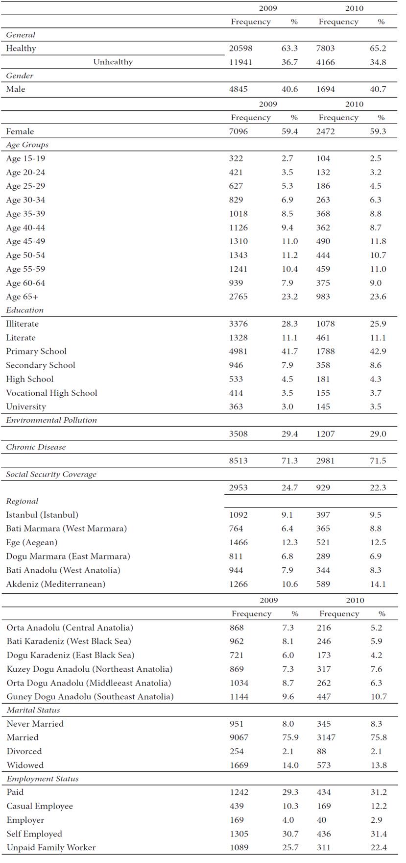
Source: Authors calculations from the data set of TurkStat for the year 2009 and 2010.
Note: The descriptive results are given only for the individuals who report themselves as unhealthy. Therefore the percentages of the subgroups show the share of the subgroup within the whole group.
Table .1 Descriptive Statistics
As can be seen from Table 1, the number of individuals (for both years) who report themselves as unhealthy are lower than that of the healthy ones. The percentages of the unhealthy individuals are around 35%. This result states that nearly one third of the society declared themselves as unhealthy. When the results of the unhealthy individuals are investigated more deeply, it is seen that women are unhealthier than the males. The ratio of women, who are reported as unhealthy, are nearly 60% whereas men are 40%.15 When we decompose individuals by age groups, it is seen that mainly older individuals report themselves as having a poor health. While 24% of the age group 65 and over individuals report poor health, it is only around 3% for the 20-24 years of age group. It is 6% for the 25-29 group. The obtained results are consistent with the theoretical expectations. The same pattern is observed when the education levels are considered. Higher education level leads to lower poor health ratio. For instance, for both years, whilst illiterate individuals who report poor health are around 28%, individuals with a university degree are only around 4%.
Those individuals who claim to be exposed to environmental pollution also claim themselves as unhealthy. These percentages are nearly around 30% for both years. Besides, as it is expected, having chronic disease leads to unhealthier individuals. Approximately, 71% of the unhealthy individuals declare that they have chronic disease. Social security coverage is engaged to utilization of health care services in Turkey. Obtained results show that without social security coverage, individuals are more likely to report themselves as unhealthy. The ratio of the individuals is around 70% for both years.
When different regions are explored more closely, it is apparent that differences in the level of development in different regions cause health differences amongst the individuals. Being relatively less developed and the lack of accessing a thorough health care, the Anatolian part (and surprisingly Aegean) of Turkey accommodates unhealthy individuals.16 The Anatolian parts of Turkey are relatively more rural in which the individuals may not be as lucky as those living in the western metropolitan parts of the country in getting more health care (for instance, accessing hospitals or medical institutions can be difficult).
These facts expose that the individuals in the eastern part of Turkey are more likely to claim poor health than the ones in the western part of Turkey for the years of 2009 and 2010. The ratio of the poor health individuals is ranging from 6% to 14% for both years across the different SR1 regional levels. While individuals in Ege (Aegean) region report the highest level of poor health for the year 2009, Akdeniz (Mediterranean) region report the highest level of poor health for the year 2010 (around 14%).
Marital status of the individuals seems to be related to age profiles. For instance, single and divorced individuals have the lowest ratio amongst other groups who see themselves as unhealthy. The married individuals have the highest percentage of reporting poor health. Actually, these results are consistent with the results of the age groups. The individuals who are not married are the ones who are relatively younger. On the contrary, the widowed individuals are more likely to be the ones within the elderly. Therefore, the results reveal that the widowed individuals have the poorer health.
The paid workers get more health care in Turkey than the other individuals. Mainly, paid workers have social security coverage and thus, they could reach more health care. However, unpaid family and self-employed workers are not able to get their needs from the health care services. The percentage of these categories are around 30%, whereas employers category is around 19% in 2009. When we compare the two selected years, it can be seen that there exists a slight deterioration of reporting poor health for all different employment categories.17
Table 2 reveals the income inequality of different regions (SR1 level) and the air pollution data for the investigated years.
Table 2 Income Inequality and Air Pollution measures for SR1 level
| 2009 | 2010 | |
|---|---|---|
| Income Inequality-Gini Coefficient | ||
| Istanbul (Istanbul) | 0.34 | 0.32 |
| Bati Marmara (West Marmara) | 0.35 | 0.34 |
| Ege (Aegean) | 0.36 | 0.32 |
| Dogu Marmara (East Marmara) | 0.35 | 0.29 |
| Bati Anadolu (West Anatolia) | 0.38 | 0.32 |
| Akdeniz (Mediterranean) | 0.38 | 0.35 |
| Orta Anadolu (Central Anatolia) | 0.37 | 0.32 |
| Bati Karadeniz (West Black Sea) | 0.36 | 0.36 |
| Dogu Karadeniz (East Black Sea) | 0.35 | 0.30 |
| Kuzey Dogu Anadolu (Northeast Anatolia) | 0.37 | 0.38 |
| Orta Dogu Anadolu (Middleeast Anatolia) | 0.37 | 0.36 |
| Guney Dogu Anadolu (Southeast Anatolia) | 0.39 | 0.38 |
| PM 10 (Particulate Matter) | ||
| Istanbul (Istanbul) | 53 | 51 |
| Bati Marmara (West Marmara) | 84 | 77.5 |
| Ege (Aegean) | 56.5 | 64.7 |
| Dogu Marmara (East Marmara) | 75 | 62.5 |
| Bati Anadolu (West Anatolia) | 72 | 65.5 |
| Akdeniz (Mediterranean) | 67 | 65 |
| Orta Anadolu (Central Anatolia) | 55 | 57 |
| Bati Karadeniz (West Black Sea) | 64 | 51.5 |
| Dogu Karadeniz (East Black Sea) | 62 | 84 |
| Kuzey Dogu Anadolu (Northeast Anatolia) | 72.5 | 64 |
| Orta Dogu Anadolu (Middleeast Anatolia) | 95.5 | 101.5 |
| Guney Dogu Anadolu (Southeast Anatolia) | 93 | 81.7 |
Source: Authors calculations from the data set of TurkStat for the years 2009 and 2010.
The results of income inequality measure of Gini coefficient show that some parts of Turkey have more unequal income distribution. For instance, Istanbul region is more equally distributed than the other regions. Actually the lower Gini coefficient of the Istanbul region might be a result of the high percentage of the labour earnings in this region. As the labor earner individuals are mainly distributed more equally than the other earners as entrepreneur and/or interest rate earners, this fact leads more equality in the region. Besides Akdeniz region has the highest value of the Gini coefficient. Actually, it is not a surprising finding surprising for Turkey. Because Akdeniz region attracts a huge amount of immigrants who are looking for more suitable job opportunities from the less developed part of the Anatolian regions of the Turkey. This is mainly because of the geographic closeness to the less developed parts and the job opportunities of this region. As they are not permanent workers, their income levels have a higher dispersion. The high migration level causes income inequality within that region. Besides, Guneydogu Anadolu (South-Eastern Anatolia) region, which is the less developed region of Turkey, also has more inequality compared to other regions. When the Turkish economy structure is taken into account, this is also consistent with the expectations.
Air pollution measure of PM10 results for different regions reveal that, more industrialized regions have higher pollution levels. As the regulation about the environmental problems is not sufficiently severe for the industries, the pollution levels at these parts have the highest figures. For instance, Batı Marmara (West Marmara) region, which is the northwest part of Turkey, has the third highest pollution level. The eastern part of Turkey, Orta Anadolu (Middle Anatolia) and Guneydogu Anadolu (Southeastern Anatolia) regions have the highest pollution level. This is mainly because of the heating choice of the individuals. As these individuals are poor they prefer to use cheaper coal to overcome their heating expenditure problems. Besides, the winter conditions of these parts are heavier than the western parts of Turkey.
Table 3a and 3b show the results of the multinomial logistic regression results for the years 2009 and 2010, respectively.
Table 3a Multinomial Logit Regression Results for the year 2009
| Variables 1 | Good Health | Fair Health | Bad Health | Very Bad Health |
|---|---|---|---|---|
| Chronic Disease | 21.76*** | 23.86*** | 25.57*** | 25.88 |
| (0.348) | (0.348) | (0.356) | (0) | |
| Social Security Coverage | 0.0157 | -0.174* | -0.423*** | -0.0209 |
| (0.0744) | (0.0965) | (0.134) | (0.351) | |
| Gender (Being a male) | -0.236*** | -0.595*** | -0.628*** | 0.151 |
| (0.0641) | (0.0890) | (0.121) | (0.341) | |
| Environmental Pollution | 0.201*** | 0.588*** | 0.597*** | 0.424 |
| (0.0608) | (0.0783) | (0.104) | (0.282) | |
| Education Level2 | ||||
| Literate | 0.229 | 0.538** | 0.593** | 0.881* |
| (0.207) | (0.227) | (0.249) | (0.461) | |
| Primary School | 0.180 | 0.0452 | -0.342* | -0.512 |
| (0.133) | (0.157) | (0.183) | (0.408) | |
| Secondary School | -0.196 | -0.440*** | -0.715*** | -1.032* |
| (0.133) | (0.171) | (0.217) | (0.554) | |
| High School | -0.178 | -0.602*** | -0.960*** | -1.519** |
| (0.143) | (0.185) | (0.246) | (0.719) | |
| Vocational High School | -0.280* | -0.833*** | -1.264*** | -1.928** |
| (0.144) | (0.191) | (0.262) | (0.830) | |
| University | -0.376*** | -1.188*** | -1.829*** | -1.790** |
| (0.146) | (0.195) | (0.284) | (0.765) | |
| Marital Status3 | ||||
| Married | 0.229*** | 0.647*** | 0.130 | -0.327 |
| (0.0743) | (0.122) | (0.183) | (0.464) | |
| Widowed | 0.974 | 1.400** | 1.085* | 0.466 |
| (0.604) | (0.625) | (0.653) | (0.989) | |
| Divorced | 0.487** | 0.904*** | 1.219*** | 0.788 |
| (0.233) | (0.293) | (0.356) | (0.886) | |
| Age Groups4 | ||||
| Age 20-24 | 0.141 | 0.745*** | 0.817** | 0.520 |
| (0.104) | (0.219) | (0.325) | (0.947) | |
| Age 25-29 | 0.138 | 0.871*** | 0.761** | 1.130 |
| (0.114) | (0.224) | (0.332) | (0.873) | |
| Age 30-34 | 0.337*** | 1.419*** | 1.273*** | 1.089 |
| (0.128) | (0.233) | (0.342) | (0.932) | |
| Age 35-39 | 0.507*** | 1.804*** | 1.599*** | 1.144 |
| (0.136) | (0.237) | (0.345) | (0.951) | |
| Age 40-44 | 0.610*** | 2.070*** | 1.725*** | 1.252 |
| (0.143) | (0.241) | (0.350) | (0.962) | |
| Age 45-49 | 0.824*** | 2.391*** | 2.228*** | 2.043** |
| (0.161) | (0.253) | (0.356) | (0.933) | |
| Age 50-54 | 0.645*** | 2.360*** | 2.145*** | 1.799* |
| (0.173) | (0.262) | (0.364) | (0.947) | |
| Age 55-59 | 0.816*** | 2.805*** | 2.679*** | 1.928* |
| (0.225) | (0.301) | (0.395) | (0.992) | |
| Age 60-64 | 1.847*** | 3.574*** | 3.469*** | 2.606** |
| (0.443) | (0.492) | (0.557) | (1.097) | |
| Age 65+ | 1.356*** | 3.230*** | 3.097*** | 2.469** |
| (0.390) | (0.443) | (0.514) | (1.050) | |
| Employment Status5 | ||||
| Paid | 0.136 | 0.213* | 0.220 | -0.656 |
| (0.0925) | (0.126) | (0.170) | (0.478) | |
| Casual Employee | 0.384*** | 0.541*** | 0.522*** | 0.0605 |
| (0.114) | (0.145) | (0.187) | (0.486) | |
| Employer | 0.184 | 0.517** | 0.763*** | -0.143 |
| (0.159) | (0.205) | (0.278) | (0.832) | |
| Self Employed | 0.151 | 0.171 | 0.255 | 0.134 |
| (0.102) | (0.127) | (0.157) | (0.373) | |
| Equivalent Household Income | -9.67e-06*** | -3.66e-05*** | -7.04e-05*** | -5.41e-05** |
| (1.84e-06) | (3.91e-06) | (7.45e-06) | (2.23e-05) | |
| Gini Coefficient | 4.269** | 11.34*** | 6.093* | -0.463 |
| (1.920) | (2.576) | (3.542) | (9.672) | |
| PM10 | -0.00398* | -0.00692** | 0.00447 | 0.00369 |
| (0.00211) | (0.00276) | (0.00360) | (0.00929) | |
| Constant | -0.204 | -5.162*** | -4.931*** | -4.934 |
| (0.674) | (0.925) | (1.286) | (3.553) | |
| Observations | 14,883 | 14,883 | 14,883 | 14,883 |
* Standard errors in parentheses *** p<0.01, ** p<0.05, * p<0.1; 1Base category is taken as very good health.; 2Base Category: illiterate; 3Base Category: Not Married; 4Base Category: Age 15-19; 5Base Category: Not Paid Family Worker. Source: Own elaboration.
Table 3b Multinomial Logit Regression Results for the year 2010
| Variables 1 | Good Health | Fair Health | Bad Health | Very Bad Health |
|---|---|---|---|---|
| Chronic Disease | 22.25 | 24.49 | 25.83 | 44.72 |
| (5,468) | (5,468) | (5,468) | (0) | |
| Social Security Coverage | 0.0435 | -0.259 | -0.127 | -0.495 |
| (0.121) | (0.159) | (0.212) | (0.771) | |
| Gender (Being a male) | -0.0359 | -0.335** | -0.188 | -1.165 |
| (0.102) | (0.147) | (0.206) | (0.737) | |
| Environmental Pollution | 0.182* | 0.405*** | 0.515*** | -1.018 |
| (0.100) | (0.132) | (0.173) | (1.067) | |
| Education Level2 | ||||
| Literate | 0.518 | 1.066*** | 1.273*** | 1.335 |
| (0.363) | (0.407) | (0.443) | (1.337) | |
| Primary School | -0.0350 | 0.189 | -0.385 | 0.758 |
| (0.215) | (0.268) | (0.311) | (1.126) | |
| Secondary School | -0.398* | -0.247 | -0.733** | -31.43 |
| (0.216) | (0.291) | (0.371) | (6.051e+06) | |
| High School | -0.308 | -0.224 | -0.883** | -31.00 |
| (0.232) | (0.311) | (0.408) | (7.431e+06) | |
| Vocational High School | -0.474** | -0.371 | -1.136** | -31.39 |
| (0.240) | (0.325) | (0.447) | (8.196e+06) | |
| University | -0.594** | -1.044*** | -1.625*** | -31.13 |
| (0.237) | (0.333) | (0.464) | (6.694e+06) | |
| Marital Status3 | ||||
| Married | 0.0502 | 0.400* | -0.653** | 18.93 |
| (0.120) | (0.204) | (0.302) | (15,968) | |
| Widowed | 0.960 | 1.360 | -0.248 | -14.50 |
| (1.042) | (1.081) | (1.150) | (2.631e+07) | |
| Divorced | -0.0890 | 0.393 | -0.874 | -13.11 |
| (0.310) | (0.421) | (0.610) | (1.358e+07) | |
| Age Groups4 | ||||
| Age 20-24 | -0.0306 | -0.000717 | 0.468 | -31.59 |
| (0.173) | (0.342) | (0.581) | (8.401e+06) | |
| Age 25-29 | 0.296 | 0.376 | 0.739 | -2.262 |
| (0.191) | (0.350) | (0.596) | (16,878) | |
| Age 30-34 | 0.659*** | 1.077*** | 1.712*** | -2.527 |
| (0.212) | (0.363) | (0.597) | (16,878) | |
| Age 35-39 | 0.901*** | 1.649*** | 2.652*** | -33.88 |
| (0.228) | (0.371) | (0.596) | (6.550e+06) | |
| Age 40-44 | 1.053*** | 1.972*** | 2.703*** | -2.146 |
| (0.246) | (0.384) | (0.611) | (16,878) | |
| Age 45-49 | 0.699*** | 1.665*** | 2.526*** | -2.106 |
| (0.247) | (0.385) | (0.607) | (16,878) | |
| Age 50-54 | 0.728*** | 1.637*** | 2.670*** | -1.614 |
| (0.277) | (0.412) | (0.629) | (16,878) | |
| Age 55-59 | 1.124*** | 2.530*** | 3.304*** | -1.017 |
| (0.389) | (0.496) | (0.693) | (16,878) | |
| Age 60-64 | 1.056** | 2.564*** | 3.781*** | -35.22 |
| (0.515) | (0.605) | (0.781) | (2.815e+07) | |
| Age 65+ | 1.400** | 3.063*** | 3.733*** | -1.229 |
| (0.642) | (0.720) | (0.879) | (16,878) | |
| Employment Status5 | ||||
| Paid | 0.0924 | 0.384* | 0.205 | 1.724 |
| (0.153) | (0.211) | (0.286) | (1.246) | |
| Casual Employee | -0.0237 | 0.390* | 0.343 | 0.926 |
| (0.176) | (0.233) | (0.303) | (1.338) | |
| Employer | -0.0264 | 0.00879 | -0.00644 | -29.31 |
| (0.265) | (0.364) | (0.513) | (1.097e+07) | |
| Self Employed | -0.00426 | 0.310 | 0.459* | 2.342** |
| (0.170) | (0.217) | (0.267) | (0.935) | |
| Equivalent Household Income | -7.99e-06** | -2.83e-05*** | -5.37e-05*** | -9.04e-05 |
| (3.59e-06) | (6.44e-06) | (1.14e-05) | (5.95e-05) | |
| Gini Coefficient | -7.980*** | -4.475* | -1.948 | -5.717 |
| (1.831) | (2.413) | (3.160) | (10.60) | |
| PM10 | 0.00672* | 0.00493 | 0.00553 | 0.000433 |
| (0.00371) | (0.00488) | (0.00620) | (0.0231) | |
| Constant | 3.459*** | -0.278 | -2.317* | -38.13 |
| (0.668) | (0.914) | (1.263) | (0) | |
| Observations | 5,551 | 5,551 | 5,551 | 5,551 |
*Standard errors in parentheses *** p<0.01, ** p<0.05, * p<0.1; 1Base category is taken as very good health; 2Base Category: illiterate; 3Base Category: Not Married; 4Base Category: Age 15-19; 5Base Category: Not Paid Family Worker. Source: Own elaboration.
If a factor were to increase the possibility of having a chronic disease, the multinomial log-odds for good health relative to very good health would be expected to increase while holding all other variables in the model constant. Since having a chronic disease is a strongly acceptable excuse to report poor health status, this is not a surprising result. If we continue to interpret the other estimated coefficients of having a chronic disease for other groups of dependent variable, these values increase by moving from good health to very bad health category. This is also an expected result, since the referent group is very good health category. For both of the years (2009 and 2010) analyzed, we observe the same pattern, noting the fact that the coefficients for 2010 are higher than the ones in 2009.
As mentioned before, social security coverage is an important factor to maintain the needs for a stable health status in Turkey. Our findings for the estimated multinomial logistic regression coefficients of having social security coverage verify this fact. In both years’ regression outcomes, it is seen that having social security coverage just leads to report good health with respect to the base outcome (very good health). Except this good health category, other negative coefficients for this variable imply that having social security coverage decreases the possibility of reporting fair or bad health.
Another important characteristic in reporting the self-health status in Turkey is gender. As it is obviously reflected to the descriptive statistics, the proportion of women reporting themselves as unhealthy surpasses the proportion of men. Hence, with respect to the base outcome, being male decreases the possibility of reporting any other category of health other than very good health. In other words, females are more prone to report bad health status than males.
Environmental pollution is also one of our primary interest variables. Individuals who are reporting environmental pollution around their neighborhood most likely report bad health status. Our estimation results for this variable confirm this linkage. The likelihood of reporting other categories of general health status increases for both years of the analysis compared to the base category, holding other variables constant.
The relation between education level and health status is about self-consciousness of individuals who try to improve their quality of life. It is a fact that educated individuals concern their health status more than less educated or uneducated ones. Moreover, it is strongly related with the level of income. Since the income level of more educated individuals are higher than less educated or uneducated individuals in Turkey, the relationship between education level and health status shows a similar pattern. Our results also affirm these priorities. The probability of reporting poor health status decreases for both 2009 and 2010 by moving from lower to higher education levels compared to the base category (illiterate).
Marital status is a demographic variable actually goes parallel with the age profile of the population in Turkey. The proportion of late marriages increases due to prolonged years for getting higher education and looking for a job. Hence, married individuals’ age profile shifts to the late 20’s or 30 onwards. Behind this demographic evolution in time, marriages also bring along economic synergies for couples in addition to emotional relationships. For divorced couples this works in reverse. Widowed individuals experience this economic struggle in their late stages of life. Considering these, it is not surprising to observe poor health status for individuals married, divorced or widowed. Our estimates for marital status do not astonish us as being married, divorced or widowed increase the probability of reporting poor health status, reserving the fact that being widowed is the worst and being married is the best among them.
Age profiles of individuals are straightforwardly related variables to self-reported health status of individuals. Age-related diseases increase the possibility of reporting poor health status. Our multinomial logistic regression outcomes acknowledge this fact. Increasing ages bring unhealthiness together.
Employment is the fundamental source of income for many individuals in Turkey. Since we cannot deny the direct relationship between income and health, employment gains importance in maintaining a better health status. A step further than that is the type of employment. Rather than being an unpaid family worker, being paid, casual or self-employed decrease the likelihood of reporting poor health. Being employer is already the best category amongst others.
Apart from individual income, household income is a crucial determinant of health. Living in a more prosperous family decreases the risks of being ill or increase the chance of finding opportunities to recover. Hence, equivalent household income is not only an indicator of overall family wellbeing, but also gives a signal for the health status of the family members. The estimates for this variable support these claims.
Our primarily concerned variables, Gini Coefficient and PM10, are also estimated within multinomial logistic regression for both years. Although there is not an empirical consensus for the impact of income inequality on health, theoretically we expect to find a negative relationship between the two. As expected, our results for Gini coefficient reveal that the increase of income inequality worsens the health outcomes of individuals. The higher income inequality leads a worsen health in the economy. The lower income level is a key factor for the disease and poor health. When the gap between income groups become greater (which means a higher income inequality), the health care treatment between these groups differ than each other. As the inequality deteoriates distribution, some of the vulnerable groups who are mainly at the lower percentile of the distribution will have difficulties to reach sufficient health care. Therefore, with the higher inequality lower income groups could not be able to reach the health care services. Actually, these findings are compatible for Turkish economy.
The results for the Gini coefficient impact on the health status for the investigated years show a different pattern. In the year 2009, the increase in income inequality increase individuals’ probability of being good and fair health compared to very good health status. This means there exists deterioration in the health status of individuals due to higher income inequality. On the contrary, in the year 2010, the higher inequality decreases the probability of being in good or fair health status. Actually this result is a confusing one, because it is not compatible with the theoretical expectations. We believe that, in the year 2010, individuals’ declaration of health status mainly affected by the mood of optimism that is created by the high economic growth in the Turkish economy.
For air pollution measure, we observe a negative relationship in our results as we expected. The higher polluted air means higher poor health for the society. According to estimation result, for the year 2009, the air pollution decreases the probability of being good and fair health.
Table 4a and 4b show nested logistic regression results of the estimated coefficients, the standard errors of the equivalent household income, the Gini coefficient, PM10 and the interaction term for these last two variables. The dependent variable for this regression analysis is a binary choice variable for health status as healthy and unhealthy.
Table 4a Nested Logit Regression Results for the year 2009
| Variables | Unhealthy |
|---|---|
| Equivalent Household Income | -3.66e-05*** |
| (1.62e-06) | |
| Gini Coefficient | 16.85*** |
| (3.703) | |
| PM10 | 0.0718*** |
| (0.0193) | |
| Interaction Term (Gini*PM10) | -0.203*** |
| (0.0524) | |
| Constant | -6.107*** |
| (1.352) | |
| Observations | 32,539 |
Standard errors in parentheses *** p<0.01, ** p<0.05, * p<0.1.
Source: Own elaboration.
Table 4b Nested Logit Regression Results for the year 2010
| Variables | Unhealthy |
|---|---|
| Equivalent Household Income | -3.22e-05*** |
| (2.63e-06) | |
| Gini Coefficient | 27.28*** |
| (4.920) | |
| PM10 | 0.127*** |
| (0.0243) | |
| Interaction Term (Gini*PM10) | -0.372*** |
| (0.0700) | |
| Constant | -9.523*** |
| (1.692) | |
| Observations | 11,969 |
Standard errors in parentheses *** p<0.01, ** p<0.05, * p<0.1.
Source: Own elaboration.
Although it has limited impact, the results suggest that the effect of PM10 on unhealthiness changes for each value of the Gini coefficient. All independent variables of the model are statistically significant for 95% confidence interval for both years. This proves the importance of all the variables on the health status of the individuals. As a matter of fact, when the results are examined, income inequality is found to have a crucial impact on the health through the air pollution measure. For both years, coefficients of the Gini coefficient variable have positive signs. This means that Gini coefficient has a positive effect on unhealthy individuals. The higher income inequality leads to higher unhealthy individuals in the population. Inequality has a modifier effect on the link between the pollution and the health for both years. The air pollution variable coefficient has also positive effect on health status. This also means that the higher air pollution the higher will be the number of unhealthy individuals. Equivalent household income level variable has a negative impact on the unhealthy individuals. This negative effect means that at the higher income levels, the health statuses of the individuals are getting better.
Conclusions
The main purpose of this paper is to reveal the impact of income inequality on the association between air pollution and health. The main motivation of this study is to investigate whether inequality plays crucial role on this relationship. In this respect, the nested and multinomial logit regression models are employed for the empirical estimations.
Since the level of income is an important indicator signaling the degree of utilization from health care services, individuals reporting poor health status cannot be assessed without considering their relative positions on the socio-economic scale. However, exogenous factors, in our case air pollution, also have the potential to be effective on the self-reported health status of individuals. In this respect, to investigate the relationship between air pollution and health, income inequality is an interesting effect modifier that needs to be analyzed. Turkey is a developing country where its regional differentiations have been obviously qualified in many studies. These differentiations are not only limited with the disparities on the level of socio-economic development, but also including diversities with respect to environmental degradation. Regional variation in the context of air quality is one of the most frequently discussed issues amongst other environmental problems. The originality of our paper stems from the pursuit of finding answers to these seemingly unrelated problems within a reasonable theoretical and empirical framework.
According to our empirical findings, in addition to socio-economic characteristics of the individuals, income inequality and air pollution measures also have statistically significant effects on the health status. The results show that, individuals who are from unequal regions report themselves as unhealthier than those of the equal regions. Moreover, particulate pollution is associated with the poor health. These findings, actually, is consistent with the theoretical background.


