


Servicios Personalizados
Revista
Articulo
 Inglés (pdf)
 Artículo en XML
 Referencias del artículo
 Enviar artículo por email
Indicadores
-
 Citado por SciELO
 -
 Accesos
Links relacionados
-
 Similares en
SciELO
Similares en
SciELO
Compartir

 Permalink
EconoQuantum
versión On-line ISSN 2007-9869versión impresa ISSN 1870-6622
EconoQuantum vol.11 no.1 Zapopan ene./jun. 2014
Articles
De facto exchange rate regimes and inflation targeting in Latin America: Some empirical evidence from the past decade
Cecilia Bermúdez1
1 Instituto de Investigaciones Económicas y Sociales del Sur (IIESS)-Consejo Nacional de Investigaciones Científicas y Técnicas (CONICET). Departamento de Economía, Universidad Nacional del Sur. E-mail address: cbermudez@uns.edu.ar
Recepción: 05/04/2013.
Aceptación: 10/01/2014.
Abstract
We estimate de facto exchange rate systems for the seven most important Latin American economies (LA-7) between 1999 and 2011. We use the methodology developed by Zeileis, Shah and Patnaik (2010) because, unlike others developed so far, it captures the "fine" structure behind the regimes and identifies structural breaks at sharp dates. We conclude that the countries listed in AL-7 have moved towards more flexible exchange rate systems, though there are differences in the degree of exchange rate flexibility between countries that have implemented inflation target schemes and those that have not.
Keywords: Latin America, exchange rate regimes, inflation targeting.
Classification JEL: F31-F33.
Resumen
Este trabajo estima los regímenes cambiarios de facto de las siete economías más importantes de América Latina (LA-7) entre 1999 y 2011. Se utiliza la metodología de Zeileis, Shah y Patnaik (2010) que, a diferencia de otras desarrolladas hasta el momento, captura la estructura "fina" de los regímenes cambiarios de facto e identifica quiebres estructurales en fechas precisas. Se concluye que los países de AL-7 han logrado converger hacia un mayor grado de flotación cambiaria de facto, aunque existen diferencias en el grado de flexibilidad cambiaria entre los países que han adoptado esquemas de metas inflacionarias y los que carecen de ellas.
Introducción
The difference between the exchange rate regime officially declared by central banks to the IMF (de jure) and the one in operation (de facto) has given rise to alternative methods to identify the observed exchange rate regimes.2 The increasing interest in assessing the functioning of exchange rates regimes stems from the fact that the empirical research based on de jure classification yield unsatisfactory results in terms of at least two issues: the effect of nominal exchange rates on real variables and the effectiveness of intermediate regimes.
The standard literature on the relevance of exchange rates supports the "classical dichotomy", so it becomes inconsequential whether countries choose fixed or floating regimes.3 Nonetheless, policy discussions, central banks' practice and a great deal of empirical literature suggest a strong link between exchange rates and real variables. However, there is no consensus about what regime a country should adopt. While the Mundellian approach argues in favor of floating regimes –because of their ability to absorb shocks–, the "nominal anchor view" fosters fixed exchange rates because they could cover a "deficit" in monetary credibility.
The relevance of exchange rates became a central topic during the nineties. Financial integration gave rise to the "bipolar view" of exchange rates, which suggested that intermediate regimes would tend to disappear, as large swings in capital flows would make them vulnerable to speculative currency attacks. As a result, it was argued that countries should move either to pure flexible regimes or to hard pegs (Eichengreen et al., 1994; Fischer, 2001).
The same argument was employed to explain the theoretical functioning of inflation targeting schemes. If the monetary authority has an inflation goal, it cannot target other indicators because it has only one policy instrument: the interest rate. Thus, only flexible exchange rates are possible within an IT framework (Agenor, 2002). This notion goes against central banks' practice and the empirical fact that foreign exchange intervention has not been abandoned completely, and has actually helped in smoothing the effects of the financial turmoil of 2008 (Schmidt-Hebbel, 2011).
However, these conclusions might have arisen from empirical work based on de jure classification of exchange rates (Edwards and Savastano, 1999; Rogoff et al., 2004). Overcoming this weakness has been the agenda of a large literature that has developed different methods to classify exchange rate regimes. By using de facto classifications, these research lines do not find evidence to support the "classical dichotomy" (Levy-Yeyati and Sturzenegger; 2003; Bailliu et al., 2001) or the "bipolar view" of exchange rate regimes (Calvo and Reinhart, 2002; Ghosh, Gulde and Wolf, 2003). Moreover, de facto intermediate regimes could turn to be effective in reducing excessive exchange rate volatility, even under IT frameworks (Chang, 2008; Edwards, 2006). Although there is a great deal of literature on de facto classifications and its consequences, most of the studies focus on emerging market economies or Asian countries. For Latin America there are a few results from panel data estimations or empirical study cases for Brazil, Chile and Mexico.
This paper makes an attempt to fill this gap in the literature by analyzing the de facto exchange rate regimes of the seven largest economies in Latin America. We are interested in addressing two issues concerning exchange rate regimes. Firstly, there might have been changes in the exchange rate regimes in the last decade that could be reflecting turns in the underlying monetary and exchange rate policies. Consequently, we attempt to match the structural breaks yielded by the model with the actual practice of the monetary authorities in each sub-period identified by the model. Secondly, these economies may have moved towards more flexible regimes, especially those that have adopted inflation targeting. In Latin America, the movement towards these schemes began in the early 1990s, but full-fledged ones were adopted only in the late 1990s and early 2000s, following the 1998 financial crisis. Therefore, we analyze if there are differences in the flexibility of the exchange rate regimes between economies that have adopted IT schemes and those that have not, and also between the inflation targeters.
To accomplish our goals, we use a data-driven method for classifying de facto exchange rate regimes developed by Zeileis, Shah and Patnaik (2010). While other classifications can only distinguish between "floaters", "intermediate" or "fixers", the method employed in this work has the advantage of yielding a continuous measure of the degree of flexibility of the exchange rate regimes, thus allowing an analysis based on a "finer structure" of the regimes.
The remainder of this paper is structured as follows. In Section De facto classifications of exchange rate regimes and IT schemes we survey the literature on de facto exchange rate regimes and their link with inflation targeting. In Section Empirical strategy we present the empirical strategy, followed by the results in Section Exchange rate regimes estimations. Section Discussion of results: exchange rate regimes in Latin America presents a discussion and interpretation of the results and, finally, we present some final remarks concerning our results.
De facto classifications of exchange rate regimes and IT schemes
There is a general consensus in the literature that de facto classifications of exchange rate regimes have yielded quite unsatisfactory results when using the de jure coding. In particular, the "bipolar view" is no longer supported when using de facto classifications, as officially pure regimes are often intervened with different purposes and results.
In this regard, Frankel (1999) and Ghosh, et al., (2003) focus on countries with regimes reported as pegs, and find that their central banks often undergo frequent devaluations in order to maintain or enhance competitiveness. Conversely, Calvo and Reinhart (2002) analyze a group of countries with de jure flexible regimes, and find that they exhibit what the authors have called "fear of floating": in countries with a high degree of financial dollarization, the monetary authority has strong incentives to intervene in the exchange rate market to reduce exchange rate volatility, which could have a negative impact on the balance sheets of the agents.
The empirical literature on inflation targeting also aims at de facto intermediate regimes to explain the adoption and functioning of idiosyncratic IT schemes in developing economies. The standard central bank practice argues that pure floating regimes are a prerequisite for adopting inflation targeting (Agenor, 2002). However, there is evidence that central banks of emerging economies tend to intervene in their foreign exchange markets, even under an IT framework. Chang (2008) reviews the experience of Latin American central banks that have adopted IT schemes, and finds that their exchange rates regimes are actually less flexible than what could be the conventional wisdom about inflation targeting. In turn, Mohanty and Klau (2004) use a standard open economy reaction function to analyze the behavior of IT central banks of emerging market economies, and show that the interest rate responds strongly to the exchange rate and, in some cases, the response is higher than that to changes in inflation or output gap.
There are also study cases for certain countries that show similar results. Hammerman (2005) runs a VAR model for Chile and Poland, and finds that Polish monetary policy has a clear break when the exchange rate as the nominal anchor is replaced by inflation targeting; yet, it was not abandoned completely. For Chile, inflation targeting was in place for the entire sample period, but there is evidence of active exchange rate policy during the international financial turmoil. In turn, Domaç and Mendoza (2004) analyze whether foreign exchange interventions by the Banks of Mexico and Turkey have been effective in reducing volatility, and whether this has helped achieving their targets. Their results suggest that foreign exchange interventions in these countries have decreased exchange rate volatility at no costs in terms of the attainment of their annual inflation objectives.
These results highlight the importance of the exchange rate as a source of shock and, therefore, the relevance of its management in emerging countries, even in those with IT schemes.
Empirical strategy
Data-driven methods for classifying exchange rate regimes are often based on algorithms that involve ad hoc assumptions and have weak statistical foundations. In this regard, we employ Zeileis et al. (2010) approach, in which a de facto exchange rate regime classification –à la Frankel-Wei– is complemented by sound inferential techniques for evaluating the stability of the regimes in terms of the regression coefficients and the error variance. The framework involves three stages: 1) setting up the econometric model; 2) testing the stability of the parameters; and 3) establishing a dating procedure.
The econometric model
We run the standard linear regression model popularized by Frankel and Wei (1994)

in which yi are the returns of the target currency and the xi are vectors of returns for a basket of c currencies –the US dollar (USD), the Japanese Yen (JPY), the British sterling pound (GBP) and the Euro (EUR)– plus a constant. For both yi and xi in (1), log-difference returns (in percent) of different currencies are used, as computed by 100·(log pi - log pi-1), where pi stands for the value of a currency at time i in a suitable numeraire.4 Frankel and Wei (1994) use the Swiss Franc as the numeraire, but in this work we choose to use Special Drawing Rights because flexible exchange rate regimes may be sensitive to the choice of the numeraire (Zeileis et al., 2010).
The interpretation of the coefficients is as follows. When a country has a fixed exchange rate, one coefficient is 1 and the remaining ones are zero, and the error variance is σ2=0 . When a country runs a pegged exchange rate against one currency, one coefficient is near 1, the remaining ones are near zero, and σ2 takes low values. With a basket peg, σ2 takes low values and the coefficients correspond to the weights of the basket. With a floating rate, σ2 is high, and the values reflect the natural current account and capital account linkages of the country. Consequently, the error variance, σ2 or alternatively, the associated R2 value, reflects the degree of pegging. R2 values near 99% are usual for fixed regimes, while lower values are obtained for floating schemes.
Testing the stability of the parameters
An obstacle in establishing the exchange rate regime is that it is often not known if and when shifts occur. These –rather than smooth transitions– are particularly important because changes in the exchange rate regime typically stem from policy interventions of the central bank.
Although structural changes techniques are well developed for OLS models, RSS-based tests, such as Bai-Perron (2003), are insensitive to changes in σ2.5 This is rather inconvenient when estimating and testing exchange rate regimes, as the error variance represents the flexibility of the exchange rate regime in operation. In this regard, we adopt Zeileis et al. (2010) alternative to explicitly include σ2 as a full parameter, by adopting a quasi-normal model with density6:

where Φ(.) is the standard normal density function. This has the full combined parameter θ = (βT,σ2)T of length k = c +2 (c currency coefficients, intercept, and variance). By adding the error variance as a full model parameter, parameter stability can be assessed jointly for β and σ2. Then the empirical estimating functions for the corresponding ML estimates are:

The stability of the parameters β and σ2 can be assessed by testing whether the empirical estimating functions  differ systematically from their zero mean. To capture systematic deviations, the empirical fluctuation process of scaled cumulative sums of empirical estimating functions is computed:

where  is allowed to be a HAC estimator of the parameters. The empirical fluctuation process (efp) –defined as the decorrelated partial sum process of the empirical estimating functions– is governed by the central limit theorem under the null hypothesis of parameter stability. If the efp crosses the theoretical boundaries, the fluctuation is improbably large, so the null is rejected. The statistic used to test this hypothesis is a double maximum statistic that allows for both identification of potential structural instability in time and independent components of the epf process:

where epfj(i/n) is an n x k array for finite samples, with i=1,...,n corresponding to time points and j=1,...,k to the independent components of the process (i.e., components of the parameter vector under the null hypothesis of stability). The epfj(i/n) which crosses some absolute critical value, can be regarded as violating the hypothesis of stability (Zeileis et al., 2010).
Dating procedure
If there is evidence for parameter instability in the regression model, the next step is to figure out when and how the parameters changed. We use Zeileis et al. (2010) modified version of the Bai-Perron's (2003) procedure for estimating the breakpoints of a linear regression. In order to exploit changes in the error variance, the authors use the same dynamic programming algorithm but based on a different additive objective function: the negative log-likelihood from a normal model.
For a fixed given number of breaks m, the optimal number of breaks (log-likelihood) can be found using standard techniques for model selection, e.g., information criteria or sequential tests. Through this, dates of structural change in the exchange rate regime are identified. For each country, a set of sub-periods are identified. In each sub-period, the regression R2 serves as a summary statistic about exchange rate flexibility. Values near 1 convey tight pegs. Floating rates take lower values.
The dataset and descriptive statistics
The dataset consists of the following 7 countries: Argentina, Brazil, Chile, Colombia, Mexico, Peru and Venezuela. We use weekly currency returns data from January, 1999, to December, 2011.7 The currencies include the US dollar, the Japanese Yen, the British sterling pound and the Euro. The Special Drawing Rights is the numeraire. The data is provided by UBC's Sauder School of Business (available at: http://fx.sauder.ubc.ca/data.html). We denote currency returns with their ISO 4217 abbreviations.
A first glance at the data evinces the peculiarities of the period under study. After decades of public deficit financed through money creation, hyperinflation episodes and exchange rate crises, LA-7 economies have achieved sustained economic growth with low inflation levels. However, as shown in Table 1, there are some differences between countries that have adopted IT schemes (Brazil, Chile, Colombia, Mexico and Peru) and those that have other monetary policy frameworks (Argentina and Venezuela). On average, inflation rates have been almost four times lower in inflation targeters (hereon ITers), while money growth is lower by half the rate of Non-IT countries (Non-ITers).
Moreover, ITers have lower inflation rates and volatility, as measured by the standard deviation of the inflation rate. However, ITers are far from being a homogeneous group in terms of foreign exchange intervention, as shown in the last column of Table 1. If intervention is associated to movements in the exchange rate –i.e., it is not only motivated by reserve accumulation– then these differences should be reflected in the degree of flexibility of the de facto exchange rates regimes. We will return to this issue when we discuss the results of our estimates.
Exchange rate regimes estimations
This Section presents the results of the exchange rate regime estimation for each country, and a summary of the behavior of the monetary authorities in each identified sub-period.
The estimation for Argentina yields five exchange rate regimes. The first one corresponds to the last years of the convertibility regime, in place since 1992. The model accurately predicts the structural change in January, 2002, when the Congress voted for the derogation of the convertibility regime.
The second period accounts for the six months that follow the initial overshooting of the exchange rate, after a sharp devaluation. The error variance of the model, σe2, is extraordinarily high, so the R2 is almost zero. During these months, Argentina experienced the most important substitution of local financial assets (money and deposits) by external assets (foreign reserves). This substitution is reflected in the nominal exchange rate, which was devaluated 260% during the first semester of 2002. The intercept, positive and significant, accounts for this sharp depreciation of the peso.
According to Frenkel and Rapetti: "...The divergent trends seem to have been reverted by July, 2002, and the exchange market became more stable" (Frenkel and Rapetti, 2007: 7). The model yields a structural change in that date, and sets the beginning of a third period with a lower variance and higher R2 that reflects the adjustments in place.8 The intercept goes far beyond the value reach in the previous period, reflecting some degree of appreciation. But this trend was stopped by the dynamic of the local financial markets: as the rates of return of local assets began to growth, Central Bank bonds rapidly became attractive substitutes to the dollar.

In line with other exchange rate characterizations, our model yields a break in August, 2004. Simkievich (2009) analyzes the 2002-2006 period and finds two regimes: 2002-2003 and 2004-2006. The author finds that in this last period, the Central Bank made a major turn in its behavior by announcing for the first time a monetary aggregate target in its Annual Monetary Program.9
A last break is found in April, 2008, when the government imposed agricultural exports taxes. This set off the demand for dollars due to political uncertainty, which meant a drastic drain in the international reserves and, thus, a significant depreciation of the peso.
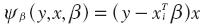
The model estimates six exchange rate regimes in Brazil, some of which coincide with the classification of Silva Jr. (2010), who estimates four regimes based on a measure of "exchange rate stress". A first break is found in January, 1999, when the Central Bank of Brazil communicated its decision of letting the exchange rate float, after almost a decade of a tight dollar peg.10
The second period begins in June, 1999, when the BCB announced the adoption of an IT scheme which has been in place ever since. The de facto indicator is consistent with an IT regime. In fact, in 2002, the BCB practiced a strong devaluation of the Real as a reaction to the inflationary shock. After the shock induced by the Argentinian crisis, the fourth period (2003-2008) reflects the IT in operation. By 2006, the BCB achieved the inflation target mainly by exchange rate appreciation, as it is reflected by the significance of the intercept in this period.
The last two regimes reflect the effects of the financial turmoil of 2008. The first months were characterized by high exchange rate volatility. The model yields a break in January, 2009, when the BCB reduced the policy interest rate from 13.75% at the beginning of the year to 11.5% in March. The degree of flexibility is lower, which reflects the BCB's foreign exchange intervention policy.
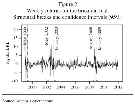
The estimates for the Chilean exchange rate regimes yield one structural change in 2008. The Central Bank of Chile has been autonomous since 1989. That same year, it adopted a hybrid IT scheme, combined with fluctuation bands for the exchange rate. The bands were meant to stabilize the functioning of the external payments system, so that they became an implicit target for the current account deficit (Céspedes, 2010).
In 1999, Chile adopted a floating exchange rate regime and made the IT scheme explicit. Since then, the BCCh intervene in the exchange market in three occasions: August, 2001, October, 2002, and April, 2008. The estimated break is placed in January, 2008, when the BCCh announced the beginning of a reserve accumulation program.
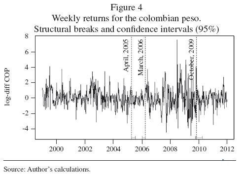
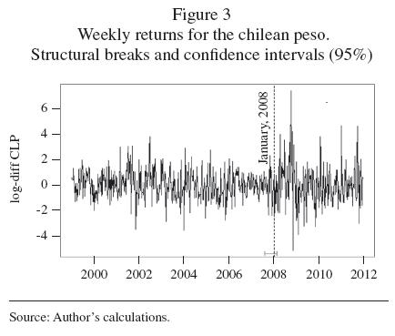
The estimated model for Colombia yields three structural breaks. Until 1999, Colombia had a hybrid scheme of monetary aggregate targets and fluctuation bands. The monetary aggregates where supposed to fluctuate within a "corridor" based on estimates of the demand for money, inflation, output growth and interest rates. As for the exchange rate, the bands were set in +/- 7%, and the Central Bank also established rules for intervention. By the late nineties, the Asian crises ended up with the defense of the bands, forced a devaluation of the Colombian Peso and pushed for the adoption of a pure floating exchange rate regime, which was combined with an IT scheme.
In 2005, the Colombian Peso registered an appreciation of 8%, which contributed to an increase in capital inflows. Additionally, commodities prices were rising and so did the terms of trade. In order to avoid an excessive appreciation of the Peso, the Central Bank practiced discretionary interventions that diminished exchange rate appreciation (Hernández Monsalve and Mesa, 2009). By March, 2006, the trend was reverted and the exchange rate reached prior levels.
According to Vargas, 2010, since 2006, the monetary policy becomes clearly anticyclical: until 2009, the Central Bank gradually increased the reference interest rate from 6% to 10% in order to reduce inflationary pressures. In turn, when the international crisis unfolded in 2008, the Central Bank reduced the interest rate to compensate the shock on the aggregate demand.
The model yields four de facto exchange rate regimes for Mexico. On December 22nd, 1994, Mexico abandoned the fluctuation bands system and adopted a pure floating exchange rate regime that remains officially to the present. Also, since 2001, the Banxico adopted an explicit IT scheme.
Between 1995 and 2003, the inflation rate decreased from 52% to 4%. Once price and financial stability have been attained, the Banxico implemented several measures conducive to the adoption of an operating interest rate target: first, the target level for banks' current account balances at the central bank (the "corto") was no longer determined based on accumulated balances but instead on daily balances; second, the Banxico decided to announce its monetary policy stance on pre-established dates.

The model yields a break at the end of 2003, when the Banxico reacted to inflationary pressures by tightening its monetary policy through an increase in the level of the "corto" and in the specific level of "monetary conditions" or interest rates (Banxico, Inflation Report, June-September, 2007). Besides, until October, 2008, US dollars were auctioned daily in order to reduce the pace of accumulation of international reserves.
The last two breaks are associated with the financial crisis of 2008. The first six months registered the highest exchange rate volatility, despite Banxico's strong intervention in the foreign exchange markets through different mechanisms (direct intervention, daily and extraordinary auctions, swap lines with the FED, among others). The Mexican Peso was depreciated in about 26% in a year, and became stable since April, 2009.
The last break estimated is placed in June, 2009. Since the second semester, the Mexican economy started a slow recovery and by the end of the year real GDP registered an annual growth of 5.5%, after the 6.1% contraction in 2008. In turn, between 2009 and 2011, there is a slight appreciation trend, which contributed to reduce the overall inflation rate from 5.30% in 2009 to 3.82% in 2011, which is still above the 3% annual target set by the monetary authorities.
The estimated model for Peru yields six breaks. The exchange rate regime for the first two periods do not match with the officially declared by the Banco Central de Reserva del Perú (BCRP), which claims to have adopted a flexible regime in 1990 and an IT scheme since 2002. Between 2002 and 2004, the monetary authorities intervened in the foreign exchange markets to counteract the excessive depreciation of the currency prompted by the uncertainty about the Brazilian electoral process.
In August, 2005, the model yields another break that is consistent with the facts described in the Memory of the BCRP: "The evolution of the nominal exchange rate shows two different dynamics in 2005. From January to August, the Sol continued to exhibit appreciation pressures (a trend that started in 2003). Since August, 2005, the exchange rate started to de-link from its fundamentals. This is explained by the recomposition of currency portfolios and the political uncertainty due to the electoral process". (BCRP, Memory 2005, pp. 39-40. Translation by the author).

Between August, 2005, and January, 2006, a sharp devaluation was triggered by massive dollar purchases by pension funds administrators, when it became public that Ollanta Humala leaded the surveys. At the beginning of the episode, the BCRP did not intervene, but later it was forced to do so in order to avoid an even greater depreciation of the local currency. Finally, at the beginning of 2006, the exchange rate was stabilized and started a slow upward trend. However, the monetary authorities' fear of floating was still very strong: despite having inflation rates under control, the BCRP decided to raise the reference interest rate by 0.25% (Alonso et al., 2010).
In October, 2009, the model yields another break. The financial crisis forced an important cut in the reference interest rate, from 6.5% in January to 1.25% in August, 2009. However, it was again set in 3% by December, 2010.
In this last period, the BCRP intervened in the foreign exchange markets in order to reduce excessive exchange rate volatility.
The model for Venezuela yields six de facto regimes that alternate hard pegs to the dollar and brief periods of floatation. In the first period, the de facto regime matches the de jure regime in place from July, 1996, to January, 2002, when Venezuela adopted a fluctuation bands system. However, the R2 is quite low. Schliesser (2004) analyses the same period and finds that the active intervention in the exchange rate market and the interest rate impeded greater movements of the exchange rate.
The second period starts in February, 2002. Since 2001, the decrease in the foreign reserves due to the fall in the oil price put pressure on the Central Bank of Venezuela, which ultimately stop defying the fluctuation bands and adopted a floating scheme, as reflected by the R2 and the extraordinary value in the error variance of this period.

On March 3, 2005, the Government of Venezuela practiced a devaluation of the Bolívar and fixed an exchange rate of Bs. 2.150. The de facto indicator shows great fixation, despite the monetary authorities not announcing the abandonment of the floating regime.
In 2008, the Bolívar was revalued at a ratio of 1 to 1000 and renamed Bolívar Fuerte. This implied just a re-scaling in the value of the currency. In January, 2010, the Government practiced a dual devaluation that reached 20% for oil-related sectors and a 100% for non-oil economic sectors.
The model yields a break at the end of 2009, due to the instability triggered by the financial crisis. During the first week of 2011, the Government announced the unification of the exchange rate system. This implied a devaluation of around 60% of the value of the currency, reflected in the extraordinarily high value of the error variance in this period.
Discussion of results: exchange rate regimes in Latin America
In this section, we discuss the results of the estimates of the de facto exchange rate regimes. Table 9 presents the de facto regime indicator –the R2– jointly with the IMF classification.11 As the R2 decreases, the regime becomes more flexible, so it is an indicator of the degree of inflexibility.
In order to make them comparable, we use IMF periodization and R2 averages for every period.
Table 9 evinces similarities and differences between both classifications:
• Argentina and Venezuela experienced periods of high and low exchange rate flexibility, but this instability is not reflected by the IMF classification.
• Mexico is classified as an "independent floater with an IT framework" by the IMF, but its de facto regime indicator, the R2, has been higher (i.e., less flexible) than that of other ITers.
• Chile is also an "independent floater with IT scheme" for the IMF, which is consistent with the de facto indicator (constant and low R2 for all the periods).
• According to the IMF, Colombia was an "independent floater" until 2004, became a "managed floater" in 2006, and went back to "free floating" in the last period. The de facto indicator also captured these changes.
• Peru was classified by the IMF as a "managed floater" and in the last period it turned to "floating". The de facto indicator partially coincides with this classification: the R2 is generally high and slightly decreases in the last period. Contrarily, Brazil went from "independent floater" to "floater" in the last period. The de facto indicator actually captures the decreasing flexibility of the exchange rate regime.
In summary, there are significant differences in the degree of flexibility between ITers and Non-ITers, which are captured by both classifications. However, our de facto estimates yield a "fine structure" of the exchange rate regimes that allows for dissimilarities also between ITers. We now turn to compare ITers with Non-ITers, and then ITers among themselves.
ITers vs. Non-ITers
Figure 8 evinces the differences in the degree of inflexibility (R2) between ITers and Non-ITers. Argentina and Venezuela are shown separately because, unlike ITers which have more or less floating systems, they do not share the same regime: Venezuela has a hard peg to the dollar occasionally interrupted by devaluations, while Argentina has a managed regime. During the period under analysis, both countries experienced large swings in the degree of flexibility of their regimes, despite the frequent interventions and controls imposed to their exchange rate markets.
Conversely, ITers have maintained a high and constant degree of flexibility over the last decade (an average R2 of around 0.30). Their exchange rate regimes have been flexible but not as volatile as what could be expected in a freely floating system. This reflects an idiosyncratic characteristic of ITers in developing regions: the role of the exchange rate is much more prominent than in advanced economies, and there is often a commitment to avoid excessive exchange rate volatility. Therefore, although the primary policy instrument is the reference interest rate, IT– central banks of developing countries also use reserve requirements and foreign exchange intervention as supplementary instruments.
The de facto flexibility in the exchange rate regimes could partially explain why ITers seem to have coped better with the commodity price and financial shocks of 2007-2009. When the crisis unfolded, ITers have already completed the phase of disinflation after the adoption of an IT regime, as shown in Table 10. Price stability may have permitted these countries to lower their interest rates and absorb part of the shocks mainly through an initial exchange rate depreciation and loss of international reserves, without triggering an exchange rate crisis, as in past episodes of external shocks (Albrieu and Fanelli, 2010).
Contrarily, Argentina and Venezuela had less room for monetary policy and exchange rate policy in 2008, as they were facing high inflation rates since the beginning of the commodity shock.
Comparison between ITers
Although ITers have quite flexible regimes, they are not pure floaters and they do not float the same way. The differences in the degree of flexibility of their regimes estimated in this work may arise from the frequency and amount of foreign exchange interventions, as shown in Figure 10.
With the exception of Chile,12 all ITers in our sample have significantly intervened in their foreign exchange markets over the last decade. Purchases were the more prevalent operation, which could imply that intervention in these countries may be associated with the avoidance of appreciation trends and also with reserve accumulation.
Brazil and Peru could be characterized as "heavy interveners". Also, our model identified many exchange rate regimes for these countries, with different degrees of flexibility, which approximately follow the pattern of interventions. These could suggest that these central banks may have certain concern about excessive exchange rate volatility. Indeed, Peru has explicitly stated this objective by setting thresholds, but Brazil has not and its intervention has been discretionary.
Conversely, in Colombia, the monetary authorities seem to have responded to appreciation trends rather than to exchange rate volatility. This is consistent with the results of our model, which shows that Colombia has an intermediate degree of flexibility.
Chile and Mexico have both made the announcement of a reserve accumulation program: Chile in April, 2008, and Mexico in February, 2010; officially, their monetary authorities have stated that these episodes of intervention had no intention to influence the exchange rate. But despite being both "low interveners", unlike the central bank of Chile, the Banxico has had a concern for exchange rate stability over the last decade, which is reflected in the quite low degree of flexibility of its de facto regime.
Concluding remarks
To assess changes in the de facto exchange rate regimes of the countries enlisted in LA7, we have used the method proposed by Zeileis et al. (2010) for estimating structural breaks in a Frankel-Wei model. The method allows testing for changes in the coefficients and also the error variance by adopting a quasi-normal density function in the Bai-Perron (2003) framework.
The empirical results suggest that there are significant differences between ITers and Non-ITers in relation to the degree of flexibility of their regimes. Moreover, tracking the regimes through the financial turmoil of 2008, the evidence shows that ITers absorbed a great part of the shock through movements in their exchange rates, without prompting an exchange rate crisis. Conversely, Argentina and Venezuela could not avoid an increase in the pace of their inflation rates, that were already high by the middle of the decade.
However, ITers were found to be less flexible than what could be expected. With the exception of Chile, ITers exhibited certain degree of "fear of floating", which may have induced them to practice interventions in order to avoid excess exchange rate volatility, appreciation trends or reserve accumulation.
A concern for the exchange rate and an operating IT scheme are not possible within the "bipolar view" framework. However, Latin American ITers seem to have managed to do so in a context of high international liquidity. Therefore, the efficiency and sustainability of this particular monetary and exchange rate framework remain to be tested under different conditions.
References
Agenor, P. (2002). "Monetary policy under flexible exchange rates: an introduction to inflation targeting". In Loayza, N. and R. Soto (eds): Inflation Targeting: Design, Performance, Challenges, Banco Central de Chile. [ Links ]
Albrieu, R. and E. Corso (2008). "Política monetaria, política fiscal y objetivos múltiples en Argentina 2002-2006". Documentos del CEDES No. 38, Buenos Aires, Argentina. [ Links ]
Alonso, G., P. Esquerra, A. Flores, L. Haman, M. Jamil and L. Silva (2010). "Política monetaria y cambiaria y estabilidad del tipo de cambio en algunos países emergentes". Borradores del Banco de la República, No. 426. [ Links ]
Backus, D. and Smith, G. (1993). "Consumption and real exchange rates in dynamic economies with non-traded goods". Journal of International Economics 35(3-4): 297–316. [ Links ]
Bai, J. and P. Perron (2003). "Computation and analysis of multiple structural change models". Journal of Applied Econometrics, 18, pp. 1-22. [ Links ]
Bailliu, J., R. Lafrance and J. Perrault (2003). "Does exchange rate policy matter for growth?" International Finance, 6: 381-414. [ Links ]
Baxter, M. and Stockman, A. (1989). "Business cycles and the exchange-rate regime: Some international evidence". Journal of Monetary Economics 23(3): 377–400. [ Links ]
Bénassy-Quéré, A., B. Coeuré and V. Valérie Mignon (2006). "On the identification of de facto currency pegs". Journal of the Japanese and International Economies 20(1): 112–27. [ Links ]
Bubula, A. and I. Otker-Robe (2002). "The evolution of exchange rate regimes since 1990: evidence from de facto policies". IMF Working Paper No. 02/155. [ Links ]
BCRP Memory (2005). At: http://www.bcrp.gob.pe/docs/Publicaciones/Memoria/2002/Memoria-BCRP-2002-2.pdf
Calvo, G., and C. Reinhart (2002). "Fear of floating". Quarterly Journal of Economics 107(2): 379–408. [ Links ]
Céspedes, L. (2010). "Experiencias de regímenes cambiarios en Chile". Banco Central de Chile Documentos Seleccionados N°86. [ Links ]
Chang, R. (2008). "Inflation targeting, reserves accumulation, and exchange rate management in Latin America". Borradores de Economía No. 487, Banco de la República de Colombia. [ Links ]
Domaç, I. and A. Mendoza (2004). "Is there room for foreign exchange interventions under an inflation targeting framework? evidence from Mexico and Turkey". World Bank Policy Research Working Paper No. 3288. [ Links ]
Edwards, S. (2006).2 The relation between exchange rates and inflation targeting revisited". NBER Working Paper No. 12163. [ Links ]
Edwards, S. and M. Savastano (1999). "Exchange rates in emerging markets: what do we know?" NBER Working Paper No. 7278. [ Links ]
Eichengreen, B., Rose, A., Wyplosz, C. (1994). "Speculative attacks on Pegged Exchange Rate: An empirical exploration with special reference to the European Monetary System". NBER Working Paper No. 4898. [ Links ]
Fischer, S. (2001). "Exchange rate regimes: is the bipolar view correct?" Journal of Economic Perspectives, 15(2): 3–24. [ Links ]
Frankel, J. (1999). "no single currency regime is right for all countries or at all times". NBER Working Paper No. 7338. [ Links ]
Frankel, J. and S. Wei (1994). "Yen bloc or dollar bloc? Exchange rate policies of the East Asian countries". In T. Ito and A. Krueger (eds.): Macroeconomic linkage: Savings, exchange rates and capital inflows. University of Chicago Press. [ Links ]
Frankel, J. and D. Xie (2009). "Estimation of de facto flexibility parameter and basket weights in evolving exchange rate regimes". NBER Working Paper No. 15620. [ Links ]
Frenkel, R. and M. Rapetti (2007). "Política cambiaria y monetaria después del colapso de la convertibilidad". Ensayos Económicos No. 46, Banco Central de la República Argentina. [ Links ]
Ghosh A.; Gulde, A. y Wolf, H. (2003). "Exchange rate regime: choices and consequences". MIT Press, Cambridge and London. [ Links ]
Girardin, E. (2011). "A de facto Asian-currency unit bloc in East Asia: it has been there but we did not look for it". Asian Development Bank Institute Working Paper No. 262. [ Links ]
Hammerman, F. (2005). "Do exchange rates matter in inflation targeting regimes? Evidence from a VAR analysis for Poland and Chile". In Langhammer, R. J. and L. Vinhas de Souza (eds): Monetary Policy and Macroeconomic Stabilization in Latin America. Springer-Verlag. [ Links ]
Hernández Monsalve, M. and R. Mesa (2009). "La experiencia colombiana bajo un régimen de flotación controlada del tipo de cambio: el papel de las intervenciones cambiarias". Lecturas de Economía, 65: 37–72. [ Links ]
Levy-Yeyati, E. and F. Sturzenegger (2003). "A de facto classification of exchange rate regimes: a methodological note". American Economic Review Vol. 93(4). [ Links ]
Mohanty, M. and M. Klau (2004). "Monetary policy rules in emerging market economies: issues and evidence". BIS Working Papers No. 149. [ Links ]
Morse, D. (1984). "An econometric analysis of the choice of daily versus monthly data". Journal of Accounting Research 22(2): 605-624. [ Links ]
Reinhart, C. and K. Rogoff (2004). "The modern history of exchange rate arrangements: a reinterpretation". The Quarterly Journal of Economics 119(1): 1-48. [ Links ]
Roger, S. (2010). "Inflation targeting at twenty: achievements and challenges". In Cobhan, D.; Eitrheim, O.; Gerlach, S. and Qvigstad, J (eds.): Twenty Years of Inflation Targeting. Lessons Learned and Future Prospects. Cambridge University Press. [ Links ]
Rogoff, K., A. Husain, A. Mody, R. Brooks and N. Oomes (2004). "Evolution and performance of exchange rate regimes". IMF Occasional Papers No. 229. [ Links ]
Silva Jr., A. (2010). "Brazilian strategy for managing the risk of foreign exchange rate exposure during a crisis". Banco Central do Brasil, Working Paper Series No. 207. [ Links ]
Schliesser, R. (2004). "Regímenes cambiarios para economías ricas en recursos naturales". Temas de política cambiaria en Venezuela. Banco Central de Venezuela. [ Links ]
Schmidt-Hebbel, K. (2011). "Los bancos centrales en América Latina: cambios, logros y desafíos", Banco de España Documentos Ocasionales No. 1102. [ Links ]
Simkievich, C. (2009). "Política de targets dobles: efectos y sostenibilidad en el Mediano plazo". Anales de la Asociación Argentina de Economía Política. [ Links ]
Vargas, H. (2010). "Exchange rate policy and inflation targeting in Colombia". Inter-American Development Bank Working Paper No. 539. [ Links ]
Zeileis, A. (2005). "A unified approach to structural change tests based on ML scores, F statistics, and OLS residuals". Econometric Reviews, 24(4): 445-466. [ Links ]
Zeileis, A., A. Shah and I. Patnaik (2010). "Testing, monitoring, and dating structural changes in exchange rate regimes". Computational Statistics & Data Analysis 54: 1696-70 [ Links ]
2 See, for instance, Bubula and Ötker-Robe (2002), Ghosh, Gulde and Wolf (2003), Levy-Yeyati and Sturzenegger (2003), Reinhart and Rogoff (2004), Bénassy-Quéré and Coeuré (2006), Frankel and Wei (1994) and Frankel and Xie (2009).
3 This view has some empirical support. See, for instance, Baxter and Stockman (1989) and Backus and Smith (1993).
4 The reason to work in terms of changes rather than levels is the likelihood of non-stationarity. Working in changes not only allows to go beyond the usual econometric concern about this series, but also permits us to include a constant term to allow for the likelihood of a trend appreciation or depreciation (a key question of interest in examining exchange rate regimes).
5 Consequently, these tests tend to yield fewer breakpoints that reflect only changes in the intercept and/or the regression coefficients. Additionally, there are other issues related with the comparability of these tests with Zeileis et al. approach. For example, if we applied the Quandt Likelihood Ratio test, we would lose the potential breakpoints at the beginning of the sample (associated with major devaluations in some countries), as the conventional choice is to trim 15% of the observations from each end of the sample. However, the results of the QLR test are available under request.
6 We use the open codes for the R system included in strucchange and fxregime packages. Available at: http://CRAN.R-project.org/ and http://R-Forge.R-project.org/.
7 The use of weekly –instead of monthly– data is proper in this case, as there are daily events that generate abnormal returns. When structural changes are present in the data, the literature uses high frequency data because of the higher power of the statistical tests. Morse (1984) examines this issue for security returns and argues: "The return effect of a shift in the coefficients is accentuated when a lower frequency is used. The increased bias and variance for monthly data occur because the structural shift operates for a longer period. No direct comparisons of t-statistics can be made because of the bias, but Type II errors would be more likely with monthly data if no adjustments were made for the bias caused by the shift in the coefficients" (Morse, 1984: 616 ).
8 According to the authors, the causes of the relative stability achieved in this period are: a) the exchange rate controls over cross-border financial transactions, implemented since March, 2002; b) the systematic intervention in the exchange market since Roberto Lavagna assumed as head of the Ministry of Economy; c) the decision to oblige Argentine exporters to liquidate export receivables over USD 1 million at the Central Bank, which enormously contributed to increase foreign reserves.
9 The Monetary Program was officially announced in June, 2003. It consisted of three quantitative monetary goals: a minimum level for foreign reserves, and a maximum level for net domestic assets and for broad monetary base.
10 The Real jumped from 1.21 to 1.52 in January, to 1.90 BRL/USD in March.
11 Until 1998, the IMF compiled the de jure exchange rate arrangements from national sources in its Annual Report on Exchange Arrangements and Exchange Restrictions. Since 1998, in response to criticism that there were significant differences between de jure and de facto policies, the IMF shifted to compiling unofficial data and started to publish its own de facto classification, available on http://www.imf.org/external/NP/mfd/er/index.aspx . We compare our de facto indicator with the IMF classification because, unlike others, it has various categories (not only fixed-floating) and it is up to date.
12 The Central Bank of Chile also intervened in 2001 and 2002, but the amounts were not significant.

