Artículos

 

Price competition in mixed strategies in markets with habit formation

 

Alejandro Tatsuo Moreno Okuno^1*

 

¹ Profesor de Economía, Universidad de Guanajuato, correo: atatsuo@hotmail.com.

 

Fecha de recepción: 21/03/2010
Aceptación: 24/08/2010

 

Abstract

I analyze competition when individuals' favorite characteristics are the characteristics of the products they have consumed in the past. I model a two–period game in which two firms compete with each other in a market of differentiated products where individuals' favorite characteristics in the second period are the characteristics of the products they consumed in the first period. In this context, firms can manipulate the distribution of preferences. If firms differentiate their products, they will separate preferences, creating the equivalent of a switching cost between products. However, if firms produce similar products, they will reduce the cost of every individual to consume the product of the other firm, increasing competition. I solve for the Subgame Perfect Nash Equilibrium of the model and I find that firms choose to differentiate their products the most possible by placing their products at the extremes of the characteristic space.

Keywords: habit–formation, oligopolistic competition, product differentiation, Hotelling's location model.

Classification JEL: D43, L11, L13.

 

Resumen

En este artículo analizo la competencia entre firmas cuando las características favoritas de los individuos son las características de los productos que han consumido en el pasado. Modelo un juego de dos periodos en el cual dos firmas compiten en un mercado de productos diferenciados, donde las características favoritas de los individuos en el segundo periodo son las características de los productos que consumieron en el primer periodo. En este caso, las firmas pueden manipular la distribución de preferencias. Si las firmas diferencian sus productos, separarán las preferencias, creando el equivalente a un costo de cambiar a otro producto. Sin embargo, si las firmas producen productos similares, reducirán el costo de todos los individuos de consumir el producto de la otra firma, incrementando la competencia. Resuelvo por el Equilibrio Perfecto de Nash en Subjuegos del modelo y encuentro que las firmas escogen diferenciarse lo más posible al colocar sus productos a los extremos del espacio de características.

 

Introduction

Psychologists have long observed that individuals can increase their enjoyment of many products just by consuming them repeatedly. Economists have formalized this phenomenon in habit–formation models. Pollak (1970) introduces utility functions that incorporate past consumption and uses them to model demand for a product as a function of previous consumption patterns. Becker and Stigler (1977) formulate a model where individuals accumulate a stock of consumption capital from past consumption that allows them to enjoy more or less (depending on whether it is a beneficially or harmfully addictive commodity) of the goods. Many other authors have extended habit–formation to a wide range of areas in the literature of economics.

However, psychologists have observed that individuals not only increase their preference for a product, but also for its characteristics. For example, in one experiment, Bertino and Beauchamp (1986) gave students food with more salt than what they normally consumed. After only 3 weeks of the higher–salt diet, these students began to develop a preference for saltier foods. After 4 weeks, students were allowed to choose the amount of salt they preferred, and it was observed that they kept on using a high concentration of salt.² It is important to note that these students not only increased their preference for the specific salty food they consumed, but they grew to prefer salty food in general. What these studies reveal is not only that the more we consume it, the more we like a product, but also that we begin to enjoy its characteristics, even when these characteristics are found in other products. Psychological studies are normally carried out over a short period, none spanning over a few weeks at most. However, in the real world, people are exposed to products for many years. Thus, habit–formation in the real world may be even stronger than what these studies revealed.

My paper seeks to analyze competition in markets with habit–formation by modeling habit–formation for the characteristics of the products. For this, I use Hotelling's model of differentiated products. Hotelling (1929) introduces competition in a market where consumers have heterogeneous preferences for the characteristics of a product. He models a characteristic space (for example, sweetness or the size of a product) where an individual's favorite level of the characteristic is uniformly distributed. Individuals want to buy one unit of a product and their utility decreases the more the characteristics of the product strays from their most preferred level. Hotelling models two firms that compete for the consumers. Hotelling's model main contribution is that it allows us to analyze competition when firms choose the design of their products.

Hotelling's model assumes that there is an infinite number of individuals with different preferences and they have to choose one of just two products. But if individuals begin to appreciate the characteristics of a product as they consume it, their preferences will become more homogenous over time, since many individuals consume the same product. In this paper, I assume that even if the initial distribution is uniform, habit–formation will lead to a distribution of preferences that is clustered around the characteristics of the goods that are available. As a result, the characteristics of the products will explain preferences as much as preferences explain the characteristics of the products.

In section II, I present my model by incorporating habit–formation into the Hotelling model. As Hotelling, I use a utility function where every individual has a favorite level of the characteristics, and their utility decreases the more the characteristics of the products they consume differ from their favorite characteristics. My model extends Hotelling's model with the inclusion of several periods and making individuals' favorite characteristics, after the initial period, a function of the characteristics of the products consumed during previous periods.

I analyze competition in section III. Given the complexity of the problem, I limit the analysis of competition to the case of two periods. In the first period, two firms enter the market; they select the level of the characteristic in their product and compete in price for consumers. Initially, individuals are uniformly distributed on the characteristic space, but in the second period, after consuming one of the products, their preferences change and their favorite level of the characteristic moves to the level of the product they consumed in the first period. In the second period, firms sell their product again. However, individuals now prefer to consume the same level of the characteristic they consumed in the first period. Since my main interest is to study competition among firms, and not how individuals manage their habit–formation, I assume that individuals are not forward looking, that is, they do not take into consideration their utility in the second period when they choose which product to consume in the first period. I solve for a Subgame Perfect Nash equilibrium of the game.

The idea that individuals prefer to consume the products they consumed in the past is closely related to the literature of switching costs. Some examples of switching costs are the costs of learning how to use a product and the need for compatibility with existing equipment, but it can also be interpreted as brand loyalty. Klemperer (1987) extended Hotelling's model to a second period in order to analyze switching costs. If individuals consume a product, they face a switching cost if they change to another product in the future. He finds that switching costs leads firms to compete more aggressively in the first period in order to "lock in" consumers for the second period, when they raise their prices for the "locked in" consumers who purchased their products in the first period.

Klemperer assumes that switching costs is exogenous to the firms and the cost to switch to a different product is independent of how different the products are. My model, instead, allows firms to choose the size of the switching cost with the design of their products. If individuals have habit–formation, their preferences will cluster around the location of the products, and firms can manipulate the distribution of preferences. If firms locate very far from each other, they will separate preferences, increasing the cost of every consumer to purchase the product of the other firm, creating the equivalent of a switching cost between products.

For example, if people grow accustomed to the flavor of a soda they consume, then they would prefer to consume the same soda and enjoy other sodas with similar flavor rather than other sodas with very different flavors. In this context, by choosing how different they make the flavor of their products, firms are choosing how costly it is for their consumers to switch to their competitor's product, and in this regard, they are choosing the switching cost.

If firms choose to locate far from each other, the results are similar to the conclusions of the switching cost literature. In the second period, consumers are "locked in" and firms can charge them a higher price, whereas in the first period, firms compete strongly in order to "lock in" consumers. However, if firms chose to locate close to each other, they will cluster the preferences of individuals, reducing every individual's cost for consuming the other firm's product, and increase competition. In this case, the results will be the opposite of a switching cost; the cost for individuals consuming the opposite firm's product is reduced for every individual, as the differentiation between products becomes smaller, thus increasing competition in both periods.

Firms may choose to differentiate in order to decrease competition in the second period, or they may choose to produce similar products to attract more consumers in the first period by making their product more attractive to consumers that are between both firms.

The result I find is that with habit–formation, both firms choose to differentiate their product as much as possible by choosing to locate at the extremes of the characteristic space.

In the same way as habit–formation affects the distribution of preferences, it affects the way in which firms compete in prices. Habit–formation creates discontinuities in the distribution of preferences, which in turn creates discontinuities in the payoffs of the firms. The price competition in the second period is in mixed strategies.

In a mixed strategies price competition, firms choose randomly among the prices in a distribution. When they choose low prices, this is interpreted in the Industrial Organization literature as a sale. My paper provides another explanation of why mixed strategies occur: habit–formation creates discontinuities in prices that compel firms to compete through mixed strategies. This differs from the switching costs literature, where firms always charge a higher price in the second period.

I conclude and offer some possible extensions in section IV.

 

The Model

Hotelling (1929) models a linear city of length one. A number of consumers live in this city and are uniformly distributed across it (for simplicity, the number of consumers is normalized to one.) There are two firms that sell a product that consumers see as identical other than the location of the firm that sells it. Consumers pay a transportation cost for each unit of distance to travel to each store and each consumer demands at most one unit of the product. Both firms choose their location and then compete in prices to attract consumers. We can also interpret this model as describing the location of preferences in a characteristic space (for example, sweetness or the size of a product) where the location of the consumers represents their favorite level of the characteristic and the location of the firms is the design of the products (the level of this characteristic in their products.) This is the interpretation I use and henceforth I use "location" as an equivalent for level of the characteristic in a product.

I expand Hotelling's model to include multiple periods in order to incorporate habit–formation. If individuals have habit–formation, they will increase their preference for products that have similar characteristics to the products they consume. My utility function represents habit–formation by assuming that individuals' favorite location is a function of the characteristics of the products she or he has consumed until that period. This utility function is defined over a multiple, possibly infinite, number of periods. In section III, I use a particular case of this utility function for the two periods' case.

Definition 1 defines a standard Hotelling's utility function.

Definition 1 An individual's utility function is given by:

where S is the surplus from consumption without taking in consideration the transportation cost, is the favorite level of the characteristic (initially distributed uniformly in the characteristic space), p_t, and l_t,are the price and the level of the characteristics of the product that the individual consumes in period t. As it is usual in the Hotelling model, I assume that S is large enough so that every consumer will want to buy a product, no matter how different it is from his favorite design.³

In order to introduce habit–formation, I assume that an individual's favorite level of the characteristics, , is a function of the characteristics of the products consumed in the previous periods; that is, . I define a property that the favorite level of the characteristic of a utility function has to possess in order to represent habit–formation.

Definition 2 An individual has habit–formation for the characteristics of the products if his favorite characteristic I* holds the following inequality:

This definition states that the distance from an individual's favorite characteristics to the characteristics of any product weakly decreases after an individual consumes that product.

In the next section I analyze competition when two firms compete for the consumers. Due to the complexity of the model, I restrict the analysis to the case of two periods.

 

Competition in the Two period case

In this section, I analyze the case where two firms compete in a game of two periods. I solve for a Subgame Perfect Nash Equilibrium of the game. Since my main interest is to study competition between firms, and not how individuals manage their habit–formation, I assume that individuals are not forward looking, that is, they do not take in consideration their utility in the second period when they choose which product to consume in the first period. I believe this assumption represents reality at a large extent, as I believe most individuals in most markets fail to realize that their preferences change with their consumption and when they do, they underestimate the change.⁴

I assume that once firms enter the market, they cannot change their location.⁵ For simplicity I assume that the marginal cost for both firms is zero and they have no capacity constraint over the number of units they can produce. For the case of two periods, an individual's utility function is given by the following definition.

Definition 3 In the first period, the utility function from consuming a product is the following:

and in the second period, the utility function is the following:

where S is the surplus from consumption without taking in consideration the transportation cost, is the initial preferred location (initially distributed uniformly about the line), l₁ is the location of the product that the individual consumes in the first period and l₂ is the location of the product that the individual consumes in the second period.

Given that I am assuming that there are only two periods, an individual's favorite characteristic in the second period is a function of the characteristic of just one product, the one that is consumed the first period. It is because of this reason that I assume that : once individuals consume for the first time, their favorite characteristics becomes the characteristics of the products they have just consumed. It is easy to see that this utility function holds the property of definition 2. Given that I am assuming that in the second period the preferences of every individual depend solely on the products they consumed in the first period, in the second period the favorite location of every individual will be concentrated at the locations of both products.

I will refer to z as the extra utility an individual gets from consuming the product he prefers regarding the one he doesn't. Using equation 2), we can see that the value of z is given by the difference between the products: .

There are two periods in the game. In the first period, firms choose their location and then firms compete in prices for the individuals that are distributed homogeneously in the characteristic space.⁶

In the second period, firms compete again in prices for consumers, but now these consumers have grown to prefer the characteristics of their products. Habit–formation creates discontinuities in the distribution of an individual's favorite characteristics that result in discontinuities in the firms' payoff functions. Because of these discontinuities, no pure–strategy Nash equilibrium exists in the second period. However, there exists an equilibrium in mixed strategies.

Firms take into consideration that their actions in the first period affect their profits in the second period. Thus, we must solve the model using backward induction. We can analyze the behavior of the firms in the first period only after we have analyzed the equilibrium in the second period.

Price Competition in Mixed Strategies in the second period

In this section, I analyze the price competition in the second period. Given the discontinuities in the firms' payoffs functions mentioned above, the Nash equilibrium is in mixed strategies. The intuition for a price competition in mixed strategies is that both firms are choosing a price randomly from a distribution of prices. Price competition in mixed strategies is often used to explain the dispersion of prices we observe in markets through time and stores. When a firm picks a low price from its distribution, we can interpret it as a sale. For example, Varian, 1980, models competition of stores that compete both for informed and uninformed consumers. Varian finds that stores compete by choosing prices randomly from a distribution. My paper provides another explanation of why the sales occur: habit–formation creates discontinuities in prices that make firms compete through mixed strategies.

In part a) of Proposition 1,1 state that there is no Nash equilibrium in pure strategies in the second period, once the distribution of preferences has become degenerate in the characteristics of the products. However, in part b) of the proposition, I state that there is a Nash equilibrium in mixed strategies. The proof of this proposition is in Appendix A.

Proposition 1: a) There's no Nash equilibrium in pure strategies in the price competition of the second period subgame; however, b) there is a Nash equilibrium in mixed strategies in the price competition of the second period subgames.

In the following part, I solve for the Nash equilibrium in mixed strategies.

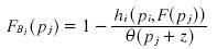
Once the distribution of preferences becomes degenerate in the characteristics of the products, the payoffs for the firms have two discontinuities. First, if the price of one firm is much higher than the price of the other firm, then no consumer (even those that consumed their product in the first period and therefore prefer it now) will buy from it. In order for this to happen, prices must be higher than the extra utility an individual gets from consuming his favorite product: z. Second, if the price of a firm is much lower than the price of the other firm (lower than z to the other firm's price), then it will attract all consumers, even those consumers who consumed the other firm's product in the first period and prefer it now. If the price of one firm is not distant from the other firm's price, not more than z, then no firm is stealing each other's consumers and their profits are yielded by the price they charge times the number of people that bought their products in the first period.

Following Osborne and Pitchik's notation (1987), I call both firms as i and j. For firm i, profits are given by the following equations (I only show the profits for one of the firms, as the profits for the other are equivalent):

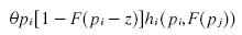
where θ is the proportion of people whose preferences coincide with the location of firm i (the proportion of people that consumed the product of firm i in the first period), p_i and p_j are the prices of firm i and firm j respectively in the second period. In order to simplify the notation, I write the prices without any subscript indicating that they are the prices of the second period.

The mixed strategies idea is that each firm's best strategy is a randomization between a distribution of prices. In order to be willing to randomize, each firm has to be indifferent between using any price in the support of their distribution. Therefore, in order to find the Nash equilibrium, we have to look for the distribution of prices for both firms that makes each other indifferent between using any price in the support of its own distribution of prices. For expositional purposes, I solve for the distribution of prices of firm j that makes firm i indifferent. The distribution of prices of firm i that makes firm j indifferent is solved in the same way. I show in the Appendix B that the support of the distribution does not have any atom or hole and its size is 2z.

Let's start by noting that if p is in the support of firm j, then p+z, p–z or both must be in the support of firm i. lf p+ z and p–z were not in the support of firm i then firm j could raise its price above p without increasing the probability of losing its consumers (or decreasing the probability of gaining more consumers); and therefore, it would raise its price.

The support of the distribution is divided into two regions: a region where firms randomize between high prices, which I will call region A, and a region where firms randomize between low prices, which I will call region B. In region A, each firm gains by charging a high price, but with some probability they lose all their consumers if the other firm's prices are low enough. In region B, each firm loses by charging a low price, but with some probability they win all the consumers if the other firm's prices are high enough (see figure 1.) In the literature of Industrial Organization, a sale is often explained as a firm picking a price in its region B.

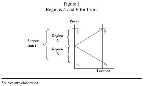
If we want that both firms pick prices randomly from their distribution, the distribution of prices of each firm has to make indifferent the other firm between using any price in its own support, in region A or in region B. When a firm is charging a high price (region A), what it cares about is the probability that the other firm's prices are low enough to steal all of its consumers; in other words, what it cares about is the other firm's distribution in Region B. For example, if firm j is considering a high price p, it cares for the probability to which firm i charges prices below p–z, as it can steal its own consumers.

Equally, when a firm is pricing low (region B), what it cares about is the probability that the other firm's prices are high enough and can steal all of the other firm's consumers; in other words, what it cares about is the other firm's distribution in Region A. For example, if firm j is considering a low price p, what it cares about is for the probability that firm i charges prices above p+z, as it will gain all of firm i's consumer. Therefore, the distribution that we need in region A is the one that makes indifferent the other firm in charging any price in its own region B and the distribution that we need in region B is the one that makes indifferent the other firm in charging any price in its own region A. Each firm's Region B ends where region A begins.

In the vertical axis of figure 1,1 show region A and region B for firm i. In the horizontal axis, I show the difference in characteristics between both products. The size of regions A and B is a function of the difference between the products of both firms.

Region B_j is associated with region A_i, and region A_j; is associated with region B_i. The distribution in region A_j is the one that makes indifferent firm i between pricing in each point in its own region B_j. The lowest point in B_iis a_i, and therefore a_i+ z is the lowest point in A_j. The distribution in region B_jis the one that makes indifferent firm i between pricing in each point in its own region A_i. The highest point in A_i is B_i, and therefore B_i – z is the highest point in B_j.

As noted above, in equation 3, profits for firm i depend on the price of firm j. Given that firm j is choosing prices randomly according to a distribution f(p_j), firm i is interested in the expected value of its profits:

where a_j is the lowest price and B_j is the highest price in the support of the distribution of firm j.

As mentioned above, the size of the support is 2z. This simplifies equation 4. If firm i chooses a high price (a price in its region A), it does not have to worry about firm j charging a much higher price, since the size of the support guarantees this. Profits for firm i if it charges a price in its region A, simplify to the following equation:

If firm i chooses a low price (a price in its region B), the size of the support guarantees that firm j won't charge a much lower price. Therefore, the profits for firm i in region B simplify to the following equation:

We want to find the cumulative distribution of prices, F(p_j), that hold constant the expected value of the profits, h_i(P_i, F(p_j)). I solve the integrals of equation 5 and 6, holding constant h_i(P_i, F(p_j)) for both regions.

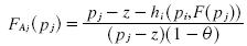
I solve first for the distribution of prices of firm j in its Region B that hold constant the expected value of the profits of firm i in its region A. Solving the integrals of equation 5 we get:

We isolate F(P_i – z), since what we are interested in finding is the distribution of prices:

Finally, I substitute p_j = p _i – z in order to have the distribution of firm j in terms of its own prices. By holding h_i(P_i, F(p_j)) constant, we get a distribution of prices in Region B for firm j that makes constant the profits for firm i. I add a subscript indicating that this is the cumulative distribution function of firmj in its own region B:

Now I find the distribution of prices for firm j in its region A that hold constant the expected value of the profits of firm i in its region B. I solve for the integrals in equation 6:

Then I isolate the distribution F(p_i + z):

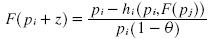
I substitute p_j = p_i +z . By holding h_i(P_i, F(p_j)) constant, we get a distribution of prices in Region A for firm j that makes constant the profits for firm i. I add a subscript indicating that this is the cumulative distribution function of firm j in its own region A:

In order to be a Cumulative Distribution Function, F(p_j) has to satisfy several conditions. The value of F(p_j) has to be one at the highest point: b_j, and zero at the lowest point: a_j. We also have the condition that expected profits are the same in both regions. From here we have 6 conditions (3 conditions for each firm) and 6 unknowns: a_i, a_j, b_i, b_j, h_i and h_j. By using these conditions we can derive that the expected value of the profits for firm i are h_i = θ(a_j + z). The intuition of this result is simple. The profits per consumer for firm i in the second period are given by the middle point of the distribution of firm j: a_j+ z, because if firm i chooses this price, firm j will not steal its consumers and firm i will not steal firm j's consumers either. The expected value of the profits in the second period are given by profits per consumer times the market share (θ): h_i = θ (a_j+ z). Finally, we need the condition that the value of F(p_j) is the same where region A ends and where region B begins.

From these conditions, we can solve for the distributions for both firms and get the values for the parameters a_i and a_j. However, I cannot find an analytical solution for the parameters and I calculate its value numerically.⁷ For example, for a market share of 0.5 for each firm and a distance between products (z) of one, the numerical value I get for a_iand a_j is 1.4142 and the expected value for the profits for firm / in the second period is: h_i = 0.5*(1.4142+l)=1.2071.

In Appendix C, I show that any price in the support of the distribution we solved above is the best response and that any deviation from this distribution is suboptimal. I do this by showing that prices above and below the support obtain lower expected profits than those prices in the support.

The Nash equilibrium in mixed strategies I just solved tells us that both firms are going to choose a price randomly from the distribution solved above. Each price in this distribution is optimal and any firm is indifferent between charging any price in those distributions.

Once having solved for the mixed strategies, I proceed by analyzing how the market share affects the expected value of the profits in the second period. The market share (θ) affects the expected profits, h_i, in two opposite directions. First, the individuals that consumed the product in the first period enjoy it more in the second period. The more individuals consumed the product in the first period the more individuals are expected to consume it in the second period. Second, more consumers for one firm mean more incentives for the other firm to price lower and steal its consumers. If one of the firms has a larger market share than the other, the distribution of prices goes down and the expected profits per consumer decreases for both firms. As we can appreciate in figure A3 (Appendix D), if θ goes from zero to seventy percent, the first effect dominates and the profits increases with more consumers. However, for θ higher than seventy percent, the second effect dominates and the profits decrease as the number of individuals that consumed the product in the first period increases.

Location and Price Competition in First Period

Once we have solved for the price equilibrium in mixed strategies in the second period, we can solve for the equilibrium in the first period. In reality there are two stages in the first period: both firms must choose first their location and then compete in prices for the consumers who are still uniformly distributed in the characteristic space.

The expected value of the total profits for each firm are given by the sum of the profits for the first period plus the present value for the expected profits for the second period:

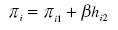
where π_il are the profits in the first period, h_i2 is the expected value of the profits in the second period for firm i and (β is a discount factor. The profits in the first period are given by the profits for the standard Hotel–ling model. The quantity that firm i sells (market share) in the standard Hotelling model is:

In the first period, the profits for firm i are given by its first period price times its market share. In the second period, as shown above, its expected profits are given by the expected profits per consumer (a_j+z)times its market share. Adding the expected profits for both periods, we have that total expected profits for firm i are given by:

The solution has to be calculated numerically as the value of a_jis calculated numerically. I solve by backward induction: I first find a price equilibrium for the second stage of the first period and then I solve for the location equilibrium in the first stage of the first period.

Price competition in the First Period

Because the solution for the second period was found numerically, the equilibrium in the first period has to be found also numerically. For this, I wrote a program that finds a Nash equilibrium for the price competition of the first period.

The basic idea is that the program finds numerically the best response by any firm to the price of the other firm, and then it finds the best response of the other firm to this best response, and then it repeatedly finds the best response to the best response it got before. By repeating this process, it eventually finds the Nash equilibrium with a degree of high precision. For example, we start by using any price for one of the firms, for example firm j. The program finds the best response of firm i to this price and then it finds the best response of firm j. Then again it finds the best response of firm i to the best response of firm j. Each time we repeat this, we get closer to the Nash Equilibrium of the stage. I repeat this until the best response of each firm to the best response of the other firm does not change. The procedure is robust to the use of any starting price, as we arrive to the same solution no matter what price we use at the beginning of the procedure.

In order to find the solution numerically, I have to assume the values for some parameters. I assume that δ =1, that is that firms do not discount the time (I tried for other values of δ without altering the results in any meaningful way). As in the previous section, I assume that the cost of production is zero. This program is able to find the solution for any particular values for the locations of each firm.

In the Nash equilibrium of the price competition of the first period, firms compete very aggressively in order to capture consumers for the second period. I find that the higher the differentiation of the products, the more aggressive the firms compete in the first period by decreasing their prices. The intuition is that habit–formation allows firms to separate individuals' preferences in the second period by separating their products. As the individuals' preferences differ more from the product of the firm they did not consume in the first period, individuals are locked in with the product of the firm they consumed in the first period, decreasing competition. Therefore, the expected profits per consumer increase in the second period with the differentiation of the products. As firms anticipate that higher differentiation brings higher expected profits in the second period, their incentive to capture more consumers by competing more aggressively in the first period increases.

As differentiation grows, competition becomes so aggressive that firms may charge negative prices: firms could have incentives to actually pay consumers to consume their products in the first period. We have to consider that this result is in the context of zero costs of production. What is important are the losses per consumer in the first period that a firm is willing to endure in its attempt to lock them for the second period. In the case of positive marginal costs of production, the price of the equilibrium moves upward, maintaining the same loss per consumer and resulting in a lower price than the marginal cost, not necessarily a negative price. This is consistent with the promotion of new products where firms many times lose money when introducing their products. In the next section, I analyze the design of the products that is given by choice of the characteristics of the products for each firm.

Choice of location in the First Period

Once solving for the price equilibrium of the second and first periods, I can solve for the choice of characteristics in the products. I look for the location for each firm that is a best response to a given location of the other firm. In order to get the best response, I calculate the expected profits for each firm for a set of locations and find the one that has highest profits. I get a new set of locations around this location and then I calculate the profits and I find the location where the highest profits are. Again I get a new set of locations around this location. I repeat this process until I get the location with the highest profits with a high degree of precision. This location is the best response of one firm to the location of the other.

By finding the location that is the best response to the other firm's location, and then finding the best response to this best response, and repeating this process numerous times, I can find a pair of locations that are best response to each other's location.

There are two effects when firms get closer to each other: the first is that they are able to attract more consumers when they get closer; as each firm gets closer, its product becomes more attractive than the product of the other firm to the consumers that are in the middle. The second effect is that competition increases in the second period if firms get closer.

I find that the second effect dominates the first one as both firms want to differentiate as much as possible, in order to decrease competition in the second period instead of gaining more consumers.

Although I solved for a Subgame Nash equilibrium, I cannot guarantee that this is the unique equilibrium of the game as there may be more solutions with different mixed strategies. I am not assuming symmetry to solve the equilibrium, however, the equilibrium I find is symmetric, as both firms locate at the same distance from the extremes for the characteristic space and both have the same distribution of prices.

 

Conclusion

I analyzed competition in markets with habit–formation by extending the idea of habit–formation to the characteristics of the products. This approach offers several advantages over the analysis of the switching cost approach, as it allows us to analyze the decision of firms for the design of their products to take advantage of habit–formation. Firms may choose to differentiate their products in order to separate individuals' preferences and decrease competition in the second period, or they may choose to produce similar products that are more attractive to consumers, even if this would cluster individuals' preferences, thus increasing competition. I find that firms choose the first option: to differentiate their products as much as possible by locating at the extremes of the characteristic space.

There are several extensions that can be made. First, if individuals do not have to consume a product to grow into prefer its characteristics (for example, if they learn the characteristics from the products that are shown in the media) then firms would take advantage of this by using habit–formation to create demand for new products by showing them in the media. This may explain advertisement, fashion and changing preferences over time.

Second, as I argue in the introduction, when individuals consume a product, they do not only increase their taste for its characteristics in a particular market, but also for the same characteristics in other markets. Thus, location and pricing choices in one market may influence the distribution of preferences in many markets. Therefore, an important extension would be to generalize the concept of habit–formation to multiple markets that share the same characteristics.

Third, I assume throughout this paper that individuals are not forward looking when choosing a product, that is that in the first period they do not take in consideration how their decisions would affect them in the second period. However, in some markets, this is highly unrealistic, as individuals use their consumption specifically to learn the characteristics of the products they want to consume in the following periods, for example, in the market of wines. I believe it would be interesting to extend my model to analyze these markets.

Finally, we have to be careful with the long run implications of my model's assumptions. Given that my analysis is just in two periods and therefore a short run analysis, we should expect that preferences return to their original state, unless we let consumers to continue consuming the same product over an indefinite number of periods. If, for example, individuals consume a different product in the second period than the one they consumed in the first period (this is possible as firms randomize their prices and sometimes attract their competitor's consumers), individuals' preferences should shift again, getting closer to the product they have just consumed. Analysis of a game of more periods is necessary in order to analyze competition in the long run.

 

References

Becker, G. and Stigler, G. (1977). "De Gustibus Non Est Disputandum." American Economic Review, Vol. 67, no. 2, pp. 76–90.         [ Links ]

Bertino, M., Beauchamp, G. K. and Engelman, K. (1982). "Long–term Reduction in Dietary Sodium Alters the Taste of Salt." American Journal of Clinical Nutrition, Vol. 36, pp. 1134–1144.         [ Links ]

Bertino, M. and Beauchamp, G. K. (1986). "Increasing Dietary Salt Alters Salt Taste Preference." Physiology and Behavior, Vol. 38, pp. 203–213.         [ Links ]

Blais, C. A.; Pangborn, R. M.; Borhani, N. O.; Ferrell, M. E, Prineas R. J. and Laing, B. (1986). "Effect of dietary sodium restriction on taste responses to sodium chloride: a longitudinal study." American Journal of Clinical Nutrition Vol. 44, pp. 232–243.         [ Links ]

Dasgupta, P. and Maskin, E. (1986). "The Existence of Equilibrium in Discontinuos Economic Games, II: Applications." Review of Economic Studies, 53, 27–41.         [ Links ]

Hotelling, H. (1929). "Stability in Competition." Economic Journal. Vol. 39, pp. 41–57.         [ Links ]

Klemperer, P. D. (1987). "The Competitiveness of Markets with Switching Costs." Rand Journal of Economics. Vol. 18, pp. 138–150.         [ Links ]

Loewenstein, G., O'Donoghue, T. and Rabin, M. (2003). "Projection Bias in Predicting Future Utility." Quarterly Journal of Economics, Vol. 118, No. 4, pp. 1209–1248.         [ Links ]

Moreno, A. T. (2008). "Habit–Formation and Monopolistic Competition." Working Paper, University of Guanajuato.         [ Links ]

Riskey, D. R., A. Parducci and G. K. Beauchamp (1979). "Effects of context in judgment of sweetness and pleasantness." Perception and Psychophysics. Vol. 26, pp. 171–76.         [ Links ]

Osborne, M. and Pitchik, C. (1987). "Equilibrium in Hotelling's Model of Spatial Competition." Econometrica, Vol: 55, Issue: 4, pp. 911–922.         [ Links ]

Pollak, R. (1970). "Habit formation and dynamic demand functions." Journal of Political Economy. Vol. 78, pp. 745–763.         [ Links ]

Varian, H. (1980). "A Model of Sales." American Economic Review. Vol. 70, No. 4.         [ Links ]

 

Notes

* Agradezco los comentarios de los revisores que ayudaron a clarificar algunos puntos. Ellos, sin embargo, no son responsables de los errores que pudieran existir en el documento.

² Other studies that have shown that variations in dietary sodium alter salt preferences are Bertino et al. (1982) and Blais et al. (1986). Another study showed that the same phenomenon occurred with the level of sugar in Kool–Aid (Riskey, Parducci and Beauchamp, 1979).

³ The article Habit–Formation and Oligopolistic Competition from Moreno (2008) does not make this assumption. In that article, this assumption is important as he does not assume a uniform distribution in the first period. In the current model, it complicates the analysis without adding anything of interest.

⁴ For example, Loewenstein et al. 2003 provide evidence of how individuals underestimate how their preferences change with changes in consumption.

⁵ This assumption is not important, but allows us to exclude the equilibria where both firms switch locations with each other in the second period.

⁶ However, as firms make two decisions in the first period, we can think of two stages in the first period: in the first stage, firms choose location, and in the second stage, they choose prices.

⁷ All the calculations and programs were solved in Mathematica and are available from the author by request.