Suplemento especial: Primer Seminario Internacional en Teoría Económica Contemporánea
Mesa 2: Finanzas y desarrollo

 

Diversified returns, aggregate wealth and varying market risk premium: testing the CAPM with data for Mexico

 

Lourdes Treviño¹

 

¹ Facultad de Economía, Universidad Autónoma de Nuevo León. Campus Mederos. E–mail: mariatr@faeco.uanl.mx, mdltv2003@yahoo.com.mx

 

Key words: CAPM, Human capital, conditional beta.

JEL Classification: G12, E30, E44.

 

Introduction

Modern portfolio theory is attributed to Markowitz (1952, 1959). Sharpe (1964), Lintner (1965), Mossin (1966) and others have utilized the choice–theoretic structure of the Markowitz model as the basis for a positive theory of equilibrium capital asset pricing under conditions of uncertainty. The Sharpe–Lintner–Black² Capital Asset Pricing Model (CAPM) is the one that financial managers use most often for assessing the risk of the cash flow from a project and for arriving at the appropriate discount rate to use in valuing the project. According to the CAPM, (a) the risk of a project is measured by the beta of the cash flow with respect to the return on the market portfolio of all assets in the economy, and (b) the relationship between required expected return and beta is linear.

The latter is known in financial literature as the static version of the CAPM, which assumes that i) all assets are readily marketable so that each investor is free to adjust his or her portfolio to an optimum, and ii) that beta is constant over time. In reality, however, every investor has nonmarketable assets, or assets that he or she will not consider marketing –either for personal choice, regulation or due to the inherent characteristics of the asset.

On the other hand, there is substantial evidence that conditional betas and expected returns depend on the nature of the information available at any point in time and vary over time.³ Specifically, there is a general agreement in the literature that stock prices vary over the business cycle.⁴ Hence, one may suspect that the market risk premium will also vary over the business cycle.

This paper is an attempt to explain some of the anomalies of the static CAPM. Therefore, following Mayers (1972), we include a measure of the return on human capital when measuring the return on aggregate wealth, and in line with Jagannathan and Wang (1996), we decompose the conditional beta to include a beta–prem sensitivity of the asset, which measures the instability of the asset's beta over the business cycle, that is, the sensitivity of conditional beta to market risk premium.

Using monthly data for the period January 1999–August 2008 for Mexico, we find that empirical support for both the static CAPM and our conditional CAPM specification. When betas and returns are allowed to vary over time by assuming that the CAPM holds period by period, the market beta remains significant. When a proxy for the return on human capital is also included in measuring the return on aggregate wealth, the explanatory power of the model is improved, and time variation effects continue to be significant. Size effects are found, but they are weak. Although the conditional model performs better than the static model, the proportion of the variation in monthly average returns that the two models explain is very similar, approximately 50 percent.

The remainder of the paper is organized as follows. Section develops the conditional CAPM specification. Section 3 and 4 describe the model specifications and data used in the study, respectively. Section 5 presents the results and section 6 concludes the paper.

 

The conditional CAPM

The Black (1972) version of the CAPM estimates the return on any asset i as

where β_i is defined as

and E(·) denotes the expectation. This version of the CAPM is called the static CAPM, since β_i is constant, or unconditional CAPM, since conditional information plays no role in determining excess returns.

Following Merton (1980), it will be assumed that the CAPM will hold in a conditional sense. Therefore, for each asset i in each period t

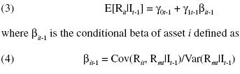
The subscript t indicates the relevant time period. R_it denotes the return on asset i in period t, and R_mt the return on the aggregate wealth portfolio of all assets in the economy in the period t. R_mt is referred to as the market return. I_t–l denotes the common information set of the investors at the end of period t–1. γ_{0 t –1} is the conditional expected return on a "zero–beta" portfolio, and γ_{1t –1} is the conditional market risk premium.

Since the aim of this study is to explain the variations in the unconditional expected return on different assets, we take the unconditional expectation of both sides of equation (3) to get

Here, γ₁, is the expected market risk premium, and , is the expected beta.⁵

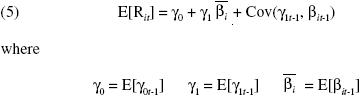
Jagannathan and Wang (1996) show that the conditional beta (which is a random variable) can be decomposed into three orthogonal parts according to the following equation

Hence, the unconditional expected return on any asset i is a linear function of its expected beta and its beta–prem sensitivity. The larger this sensitivity, the larger the variability of the above second part of the conditional beta. In this sense, the beta–prem sensitivity of an asset measures the instability of the asset's beta over the business cycle.

It is assumed that the market risk premium is a linear function of the market premium (in this case, the spread between corporate and government rate on short term debt). The premium beta is then defined as

Following Mayers' (1972) work, our proxy for the market return includes a measure of return on human capital.⁶ The specification of the CAPM explicitly accommodating human capital would have two factors as a proxy for the return on the market portfolio: the return on a value–weighted stock index, R_t^vw, and the labor income growth, R_t^labor. Therefore, it is assumed that the market return is a linear function of R_t^vwand R_t^labor, and that there are some constants , such that

Additionally, we define the value–weighted stock index beta and the labor beta, respectively, as

All the above discussion leads us to specify the model for this empirical study as

according to which the unconditional expected return on any asset is a linear function of its three betas only.

 

Econometric tests

We examine whether any residual effects exist by including the logarithm of the market value of the portfolio into the model in equation

where MV is the size of the portfolio measured as the logarithm of the weighted average of the market capitalization (in million pesos) of the individual stocks forming portfolio i in month t.⁷

The subscript t in equation (13) denotes month. Instead of using the common procedure of calculating the average of the 116 monthly–return observations (January 1999–August 2008) and use that as the only observation for portfolio i in the database, we chose a recursive analysis in which we calculate the average monthly returns for each of the 15 portfolios using the returns for the previous 24 months. We repeated this procedure month by month accounting for the rebalancing of the portfolios. By doing so, we are in fact back–testing the conditional (and static) CAPM. That is, we are testing if the model can explain the average of monthly past returns of the portfolios using present and past information.⁸

The betas of equation (13) are recalculated for each observation us–ing the information for the previous 24 months.⁹ The values for β_it^prem used in the regressions are the part of this beta that is orthogonal to a constant and β_it^vw.¹⁰ Similarly, the values used for β_it^labor are the part of this beta that is orthogonal to a constant, β_it^vw, and β_it^prem.¹¹

The unconditional models in equations (12) and (13) are estimated using the Least Squares Dummy Variable (LSDV) and within effect estimation methods for the time–series cross–sectional data described below. We use fixed effects regressions and robust standard errors. The models were estimated using Stata. Since the model in equation (13) nests the static CAPM (of equation 1) as a special case, it facilitates the comparison of the two models.¹² For comparing the relative performance of the different empirical specifications, we use the R² in the panel data regression as an intuitive measure, which shows the fraction of the variation of monthly returns that can be explained by the model. ¹³

 

Data

Monthly average returns were computed for the period January 1999–August 2008 for 15 diversifed portfolios of Mexican common stocks. The individual stocks were then combined to form portfolios without allowing borrowing or lending at the risk–free interest rate. The portfolios were selected such that they lie on the mean–variance (efficient) frontier and the stocks used to construct the portfolios were those most actively traded in the Mexican Stock Exchange (BMV) for the period of study, on daily basis. The monthly return on each portfolio is the weighted average of the current monthly returns on the individual stocks forming the portfolio. The monthly average return is calculated using the returns on the previous 24 months. The average return on each of these portfolios is then computed for the following 12 calendar months. The selection procedure is repeated each calendar year, thereby allowing for the rebalancing of the portfolios. This gives a time series of monthly returns with 116 observations for each of the 15 portfolios. The return on the value–weighted stock index is measured as the monthly return on the Mexican Stock Exchange Index (Índice de Precios y Cotizaciones, IPC). Monthly returns are calculated as the change in the logarithm of the closing prices of consecutive months. Closing prices are taken from Economatica database.

We chose the spread between the short–term rate of corporate debt and the 6–month Treasury bill rate as a proxy for the market risk premium. The short–term corporate debt rate is taken from Mexico's Central Bank (Banco de México) statistics and the 6–month Treasury bill rate is taken from infosel financiero database.

The return on human capital is proxied by the monthly rate of growth on minimum labor income in Mexico, which is an average of the minimum daily salary paid in the country. Data are taken from the índice Real de Salario Mínimo General published by Banco de México. We use a two–month moving average in the per capita labor income index to minimize the influence of measurement errors. All rates of return used are in real terms.

 

Empirical Results

The static model proves significant and explains about 47 percent of return variations. The estimation results for the conditional CAPM model including human capital are presented in Panel A of Table 1. The estimated value of c_labor is significantly different from zero at the 1 percent level. Compared to the static CAPM model, both, c_vw and c _prem remain significant and show the expected positive sign. When size is added to the model one can see that size does not really explain what is left unexplained by this model after controlling for sampling errors. The R² of 48.40 percent this model shows an improvement compared to the unconditional CAPM, and although it explains almost half of the variation of the average returns, there remains a great deal of variation that the model leaves unexplained, at least for the sample employed.

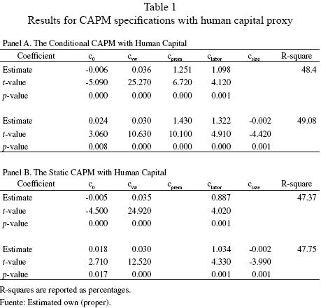
When size is added to the specification, all beta coefficients present the expected sign. On the other hand, the estimated value of the average zero–beta rate (c₀) is rather high when compared to the monthly average real rate of return of CETE28 for the period of study (0.34 percent).¹⁴ Hence, there is cause for concern even though our conditional CAPM specification does slightly better than the static CAPM in explaining the time–series cross–section of monthly average returns.

In order to determine whether human capital return is the driving force behind the results, the following model is examined:

where the static specification of the CAPM is augmented by the growth rate of minimum labor income, which is included in the proxy for the market return. The estimated results for this specification are presented in Panel B of Table 1. The coefficient corresponding to the growth rate of labor income is significant. Judging from the R², we can see that this specification explains only a slightly higher proportion of the monthly average returns as the static CAPM, and that there is only a weak residual size effect. This suggests that it is necessary to allow for time variations in betas as well in order to explain the time–series cross–section of monthly returns in stock portfolios.

 

Concluding remarks

Using data for the Mexican stock market, we find empirical support for our conditional CAPM specification. When betas and returns are allowed to vary over time by assuming that the CAPM holds period by period, the market beta and size effects remain significant. When a proxy for the return on human capital is also included in measuring the return on aggregate wealth, the explanatory power of the model is improved, and size and time variation effects continue to be significant. Although the conditional model performs better than the static model, the proportion of the time–series cross–section monthly returns that is explained by both specifications is very similar and close to 50 percent. We, therefore, reject the fat–relation between expected returns and market betas as empirical evidence in favor of the static CAPM, but did not find evidence supporting previous claims that the conditional CAPM performs substantially better than the static CAPM. In any case, the conditional model does just as well as the static model.

 

References

Ang, A. and J. Chen (2007). CAPM over the long run: 1926–2001, Journal of Empirical Finance. 14(1), 1–40.         [ Links ]

Black, F. (1972). Capital market equilibrium with restricted borrowing, Journal of Business, 45, 444–455.         [ Links ]

Bollerslev, T, R. F. Engle, and J. M. Wooldridge (1988). A capital asset pricing model with time varying covariances, Journal of Political Economy, 96, 116–131.         [ Links ]

Campbell, J. Y., and T. Vuolteenaho (2004). Bad beta, good beta, American Economic Review, 94, 1249–1275.         [ Links ]

Chen, N. F. (1991). Financial investment opportunities and the macro–economy, Journal of Finance, 46, 529–554.         [ Links ]

Fama, E. F. and K. French (1989). Business conditions and expected returns on stocks and bonds, Journal of Financial Economics, 25, 23–50.         [ Links ]

Fama, E. F. and K. French (1997). Industry costs of equity, Journal of Financial Economics, 43, 153–193.         [ Links ]

Ferson, W. E., and C. R. Harvey (1991). The variation of economic risk premiums, Journal of Political Economy, 99, 385–415.         [ Links ]

Harvey, C. R. (1989). Time–varying conditional covariances in tests of asset pricing models, Journal of Financial Economics, 24, 289–317.         [ Links ]

Harvey, C. R. (2001). The specification of conditional expectations, Journal of Empirical Finance, 8, 573–637.         [ Links ]

Jagannathan, R. and Z. Wang (1996). The conditional CAPM and the cross–section of expected returns. The Journal of Finance, 51(1), 3–53.         [ Links ]

Jostova, G. and A. Philipov (2005). Bayesian analysis of stochastic betas, Journal of Financial and Quantitative Analysis, 40, 747–778.         [ Links ]

Keim, D. B. and R. F. Stambaugh (1986). Predicting returns in the stock and bond markets, Journal of Financial Economics, 17, 357–390.         [ Links ]

Lettau, M. and S. Ludvigson (2001). Resurrecting the (C) CAPM: A cross–sectional test when risk premia are timevarying, Journal of Political Economy, 109, 1238–1287.         [ Links ]

Lewellen, J. and S. Nagel (2006). The conditional CAPM does not explain asset–pricing anomalies, Journal of Financial Economics, 82, 289–314.         [ Links ]

Lintner, J. (1965). The valuation of risk assets and the selection of risky investments in stock portfolios and capital budgets, Review of Economics and Statistics. 47(1), 13–37.         [ Links ]

Mandelker, J. (1974). Risk and returns: the case of merging firms, Journal of Financial Economics, 4, 303–335.         [ Links ]

Markowitz, H. M. (1952). Portfolio selection. Journal of Finance VII. 77–91.         [ Links ]

Markowitz, H. M. (1959). Portfolio selection: Efficient diversification of investments, Cowles Foundation Monograph No. 16 (John Wiley. New York).         [ Links ]

Mayers, D. (1972). Non–marketable assets and capital market equilibrium under uncertainty, in M.C. Jensen, ed., Studies in the theory of capital markets (Praeger, New York), 223–248.         [ Links ]

Merton, R. C. (1980). On estimating the expected return on the market: An exploratory investigation, Journal of Financial Economics, 8, 323–361.         [ Links ]

Mossin, J. (1966). Equilibrium in a capital asset market, Econometrica, XXXIV, 768–783.         [ Links ]

Petkova, R., and L. Zhang. (2005). Is value riskier than growth? Journal of Financial Economics, 78, 187–202.         [ Links ]

Shanken, J. (1990). Intertemporal asset pricing: An empirical investigation, Journal of Econometrics, 45, 99–120.         [ Links ]

Shanken, J. (1992). On the estimation of beta–pricing models, Review of Financial Studies, 5, 1–33.         [ Links ]

Sharpe, W. F. (1964). Capital asset prices: A theory of market equilibrium under conditions of risk, Journal of Finance, 19(3), 425–442.         [ Links ]

Stambaugh, R. F (1982). On the exclusion of assets from tests of the two–parameter model: A sensitivity analysis, Journal of Financial Economics, 10, 237–268.         [ Links ]

Treviño, L. (2009). How are stock Market returns affected by human capital investments? Testing the CAPM for Mexico, Working Paper, Centro de Investigaciones Económicas, Universidad Autónoma de Nuevo León. Monterrey, México, Mimeo.         [ Links ]

 

Notas

² See Sharpe (1964), Lintner (1965) and Black (1972).

³ See, for instance, Bollerslev, Engle and Wooldridge (1988), Harvey (1989, 2001), Shanken (1990, 1992), Ferson and Harvey (1991, 1999), Fama and French (1997), Lettau and Ludvigson (2001), Campbell and Vuolteenaho (2004), Jostova and Philipov (2005), Petkova and Zhang (2005), Lewellen and Nagel (2006), and Ang and Chen (2007).

⁴ Keim and Stambaugh (1986), Fama and French (1989), and Chen (1991) provide empirical evidence that supports this view.

⁵ Note that expected betas are not the same as unconditional betas.

⁶ The idea that stocks form only a small part of the total wealth is also shared by Stambaugh (1982), Diaz–Gimenez (1992) and Jagannathan and Wang (1996).

⁷ Market capitalization values are taken from Economatica and are used in constant terms as of August 31, 2008.

⁸ Treviño (2009) provides a forward–testing study for the CAPM using monthly returns for Mexico on the same portfolios analyzed here.

⁹ Using the common procedure of averaging monthly returns for each portfolio would reduce drastically the sample size hindering us from making inferences from the results.

¹⁰ We estimated equation (1), the static CAPM, and regressed its residuals to a constant, the market beta, β_it^vw, and the beta–prem, β_it^prem. The coefficients of beta–prem in the second regression are the orthogonal part mentioned.

¹¹ This allows to test for the isolated effect of β_it^prem and β_it^labor in our models.

¹² Note, however, the change in notation for γ₀, γ₁and β_i to c₀, c_vw and β_i^vw between models (1) and (13).

¹³ The .xtreg command of Stata produces the correct parameter estimates and adjusted standard errors, but does not adjust the R square. The adjusted R square was obtained by using the .areg command.

¹⁴ CETE28 is the Treasury bill of the Mexican sovereign government with a 28–day maturity, which is the one–month risk–free rate of return in Mexico.