Suplemento especial: Primer Seminario Internacional en Teoría Económica Contemporánea
Mesa 1: Economía internacional y desarrollo

 

International portfolio choice, exchange rate and systemic risks

 

J. Miguel Torres¹

 

¹ Banco Nacional de México. E–mail: jmtorresg@banamex.com

 

Introduction

We study the problem of an investor who wants to hold a diversifed global portfolio. We extend the existing literature by the joint consideration of two fundamental aspects of the international capital markets: the existence of the exchange rate risk; and the empirical fact that high–volatility events occur, and that these tend to occur at the same time across countries (henceforth called systemic risk).

We develop a model of the international capital market using the intertemporal model of Merton (1971, 1973).

 

International portfolio choice

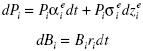
We consider an investor who acts to maximize the expected value of the payoff at terminal time T > t, where W is his financial wealth and γ is risk aversion. The investor can allocate funds across assets of n countries. In each country there are two assets: stocks, with price P_i , and riskless short–term bonds, with price B_i . Price dynamics in local currencies are described by the diffusions.

Let us pick country n as the reference country. The process of the price of one unit of currency i in terms of currency n, S_i , is the jump diffusion

z^e_i and z^s_i are Brownian motions.

Common jump dQ allows for systemic discontinuous changes in currency returns. Its occurrence is a Poisson process with rate λ , and it takes S_i . to S_i ( l+J_i ).

Let e_i and d_i be the fractions of wealth invested in stocks and bonds of country i, respectively. Also, let y_i = e_i + d_i , for i= l,…, n–l. Then the accumulation equation can be written as

The transformation induced by y_i ≡ e_i+ d_i , has an attractive intuition: whereas e_i refers to an investment protected against exchange rate risk, y_i indicates a speculative position in the currency of that country.

 

The effects of jumps on currency hedging

We consider an investing setting where the investor can allocate funds across assets of only two countries. Also, we set the coefficient of risk aversion at 2. Finally, just for the sake of easing notation, we omit the subscripts from e_i , y₁, and J₁. If ƒ (J) denotes the probability density of J, the optimal currency position is given by the solution to the following equation:

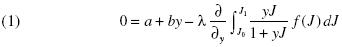
where

Whereas the term in coefficient a captures deviations from the UIP, the terms and reflect the value of currency 1 as a hedge against shifts in returns of stocks 2 and 1. Coefficient b exhibits the volatility of the price of currency 1.

We assume that J can only take two values: 0 with probability (1 – p), and k with probability p. Using 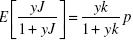and equation 1 we get that the optimum is given by the solution to the following cubic equation:

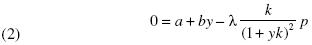
The binomial probability density has two degrees of freedom: k, the jump amplitude, and p.

In figures 1 – 3 we characterize the solutions of equation 2 for the following parameter arrangements:

1. Case I: a = – 0.50, b=0.75.

2. Case II: a = – 0.25, b=0.75.

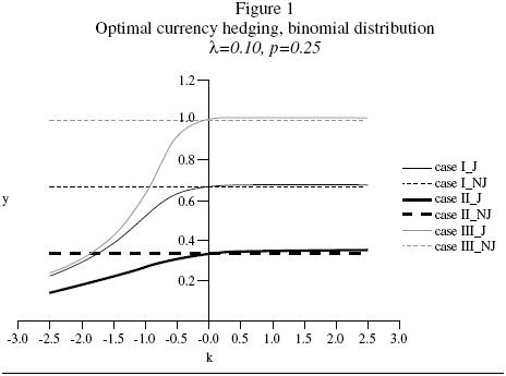
The first and the second cases are meant to illustrate the effects of changes in the premium on currency 1 or in its value as a hedge against shifts in stock returns. Recall that while increasing the premium lowers a, decreasing the hedging attractiveness raises it.

3. Case III: a=–0.50, b=0.50.

There is a direct relationship between b and the volatility of the currency price, and with cases one and three we aim to examine variations in the volatility measure.

In these figures 1 – 3, J and NJ denote currency hedging with and without jumps, respectively. We study equation 2 as a function of the jump amplitude in graph 1. The differences between the first and the other two cases are very intuitive. The second case suggests that the demand for currency 1 increases with its premium and decreases with its correlation with stocks. The third case shows that there is an inverse relationship between the volatility of the currency and its attractiveness.

While it comes as no surprise that positive (negative) jumps appear to increase (decrease) currency demand always, the asymmetric nature of the effect of the sign of the jump amplitude on the level of currency hedging is striking: compared with the effects of potential negative rare events on portfolio choice, the possibility of positive jumps has relatively negligible consequences. Indeed, larger and larger jumps need not make currency 1 more appealing. Further, optimal currency demand goes to the optimum in the absence of jumps when k goes to infinity. Intuitively, the reason is that while the mean of the jump amplitude increases linearly with k, its variance grows at a quadratic rate. A mechanical argument goes as follows. If y always remains significantly different from zero as k gets larger and larger, then the term should become or, using L'Hospital's rule, zero. Therefore, we should only be left with 0 = a+by, i.e. the optimality condition for the non–jump case.

Even though negative values of k hurt currency demand twice (low mean, high variance), equation 2 suggests that it does not become negative but vanishes as k becomes an infinitely large negative number. A heuristic mechanical argument goes as follows. If y also remained significantly different from zero as , then the L'Hospital's–rule argument we used above would also imply our being back to the same optimal hedging–level of the non–jump case. Thus, the counterintuitive character of this result lead us to argue that y vanishes as k becomes an infinitely large negative number. This explanation is consistent with what we observe in graph 1.

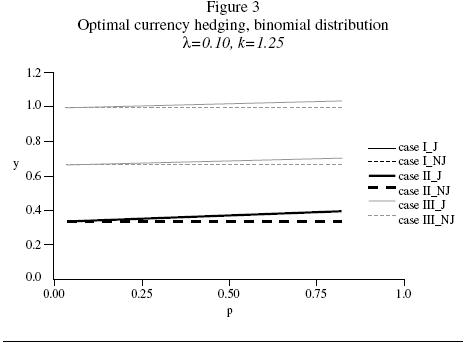
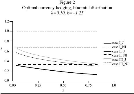
We analyze equation 2 as a function of p in figures 2 and 3. Currency demand is always decreasing (increasing) in p for negative (positive) values of k. For negative k and small p, this result is driven by two forces pointing in the same direction: decreasing mean and increasing variance. On the other hand, although the variance term is decreasing in p for p larger than ½ , its concavity makes it increasingly decreasing in p, and this should help explain the dominance in graph 2 of the expected value term, whose growth is linear (Similar arguments can be used to explain why for positive k and large p the effects of jumps on currency hedging become more noticeable for larger p, as figure 3 shows).

 

The effects of systemic risk on currency hedging

We examine the case of an investor who is fully invested in domestic equities and is considering whether exposure to multiple currencies would help reduce the volatility of his portfolio return. We set the coefficient of risk aversion at 2 again. The jump magnitudes of the two foreign currencies are assumed to be identical, and we call their common value J. Necessary optimality conditions are that at each point in time

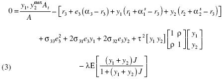
Using the spectral decomposition of the matrix , we can re–express problem 3 as follows

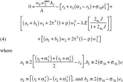
a₁ can be seen as average excess return on currencies over the domestic riskless rate. Likewise, b₁ is the average covariance between domestic–stock returns and currency appreciation. On the other hand, a₂ is the expected excess return of currency 1 over currency 2. Similarly, b₂ is the difference in covariance between domestic–stock returns and currency appreciation.

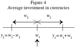
The solution of the problem in terms of the new variables w₁ and w₂ has an attractive economic intuition:

Let us now assume that J, the jump amplitude, can only take two values: 0 with probability (1 – p), and with probability ρ.In this case the expectation becomes . We can use this results and equations 4 to get that the optimum is given by the solution to the following equations:

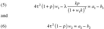
Overall exposure to currencies

w₁ is increasing in (a₁ – b₁), λ, and p; and decreasing in τ²(1+ρ). Also, the relationship between w₁ and k needs not being monotone.

Recall that a₁ is average excess return on currencies over the domestic risk–less rate, and b₁ is average covariance between domestic–stock returns and currency appreciation. Therefore, equation 5 tells us that overall currency demand has a myopic component increasing in expected excess returns on currencies, and a hedging part decreasing with the covariance between domestic–stock returns and currency appreciation.

τ²(1+ρ) embodies the covariance structure of the diffusion part of the currency processes. The effect of τ² is hardly surprising: in our setting, both currencies become riskier as we increase τ². Thus, they become less attractive for a risk–averse investor. The negative relationship between w₁ and ρ is more subtle: it mirrors the fact that w₁ is an equally weighted portfolio of the two foreign currencies. With its variance being proportional to (1+p), its attractiveness languishes when ρ increases. Intuitively, a higher ρ reduces the gains from diversification.

Optimal w₁ changes monotonically with λ and p, and the direction of the change is given by the sign of k. The intuition is simple: making discontinuous positive (negative) changes more frequent, renders foreign currencies more (less) attractive. Incidentally, under our probability density specification, λ and p are observational equivalent.

The effects of k on the optimal choice of w₁ are ambiguous. There are two competing forces. On the one hand, larger jumps only imply larger gains, in this way raising the demand for currencies. On the other hand, the variance of the jump amplitude increases with the absolute value of k, thus discouraging the asset demand.

 

Relative currency demand

From equation 6, relative currency demand, w₂, is given by provided that ρ ≠ 1.

Recall that a₂ is the expected excess return of currency 1 over currency 2, and b₂ is the difference in covariance between domestic–stock returns and currency appreciation. Therefore, relative demand for currency 1 is increasing in a₂ (myopic part). Also, the currency with the largest covariance with stock returns will experience the lowest demand as a vehicle to hedge against shifts in stock returns (hedging component).

Like w₁, optimal w₂ is a decreasing function of τ². The intuition is as follows: the diffusion term of both currencies share a common variance, τ². As τ² increases both price processes become noisier, making it harder to differentiate them. Therefore, the difference in demand between the currencies tends to blur.

The relationship between w₂ and ρ is rather subtle. Intuitively, as ρ rises, it should become increasingly difficult to tell apart the two foreign currencies. Therefore, we should become indifferent between currencies 1 and 2, i.e. we should expect w₂ to approach zero.

 

Conclusions

International asset returns are characterized by jumps occurring at the same time across countries, leading to return distributions that have fat tails. We formulate a model of the international capital market to capture these empirical properties, and then investigate the question of optimal currency hedging when currency returns have these features.

The main result from our analysis of the incorporation of systemic risk is that even in minimal models with jumps, the risk of contagion can produce complex effects on currency hedging. Although it comes as no surprise that positive (negative) jumps increase (decrease) currency demand, the asymmetric nature of the effect of the sign of the jumps on the level of currency hedging is striking: compared with the effects of potential negative rare events, the possibility of positive jumps have relatively negligible consequences.