Suplemento especial: Primer Seminario Internacional en Teoría Económica Contemporánea
Mesa 1: Economía internacional y desarrollo

 

A modified version of Solow–Ramsey model using Richard's growth function

 

Leobardo Plata Pérez^*, Eduardo Calderón^{1 **}

 

¹ Facultad de Economía de la Universidad Autónoma de San Luis Potosí. E–mail: ^*lplata@uaslp.mx; ^**jecalderon@colmex.mx.

 

Abstract

We investigate the consequences of introducing Richard's Growth function as a production function in Solow–Swan and Ramsey models. Poverty traps appear in a natural manner.

JEL Classification: O41, C61.

 

Introduction

In this paper, we modify two of the foundational models of economic growth theory: the Solow–Swan model and the Ramsey model. We make the same assumptions that appeared in the original works, except the one that refers to the neoclassical production technology. Instead, we introduce a Richard's growth function. This change permits us to model the growing process with increasing returns when the use of capital per capita is low and decreasing returns when the production factor is used in large quantities.

Richard's function has been used to model growth processes in biology. This function generalizes Logistic function and permits to change the inflexion point. Our approach is consistent with the microeconomic concept "the three steps of production", which appears in well known textbooks like Call & Holahan (1983) or Pindyck & Rubinfeld (1992). The existence of poverty traps is obtained with technologies beginning with increasing returns. The steady–state presented in Solow (1956) and Swan (1956) models are obtained as a special case of this approach. We present four types of equilibrium in the case of the Solow– Swan model. We introduce Richards's function in the model of Ramsey (1928) too. The typical saddle point appears as equilibrium in this case.

 

Generalized Solow's model

Let us assume the Solow model (Barro and Sala–i–Martin, 2004, present the standard formalization of this framework). We introduce Richard's production function as follows.

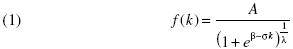
All parameters are greater than cero f(0)>0 means that there is some free production, A is the limit of f (k) when k goes to infinity. The function is always increasing in k, it is convex when k ≤ k_inf and concave when k ≥ k_inf. The point k=k_inf is the inflection point which represents the change from increasing returns to decreasing returns. Instead of the classical Inada conditions 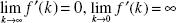we now have that the first condition is the same but the second becomes f '(0)>0. The fundamental equation is now:

From equation (2) we can obtain four cases of equilibrium.

Case 1: Solow's model ( k_inf ≤ 0 )

This case appears when the fundamental equation has only one equilibrium point. This can occur when the technology always presents decreasing returns. The equilibrium is a stable point. One example of this is obtained in the case of A = 100; s = 0.3; β = ln3; σ = 2; λ = 3; δ= 0.1; η = 0.025

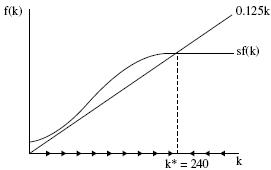
Case 2: Equilibrium with fluctuations in the economic growth rate (k_inf > 0, good equilibrium)

The inflection point is greater than zero, economic growth rate presents fluctuations before reaching the unique stable steady state, which is obtained at high level of production. One example is obtained with the following values of parameters: A = 100; s = 0.3; β= 25; σ = 2; λ= 5; δ= 0.1; η=0.025

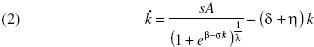
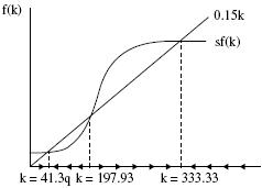
Case 3: Poverty traps (k_inf > 0, multiple equilibriums)

The inflection point is greater than cero but the economy presents several equilibriums. It is easy to check that under our assumptions there are only three equilibrium points. Two of them are locally stable and the one in the middle is locally unstable. The first equilibrium that is greater than zero is a poverty trap. Only increasing the output could allow to leave the poverty trap. In this case, the following values can give this result, A = 150; s = 0.3; β= 25; σ= 0.1; λ= 10; δ= 0.1; η=0.05

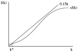
Case 4: Third world in the third world: (k_inf > 0, bad equilibrium)

This case appears when we have only one equilibrium but δ+η is very large compared to marginal returns of f (k). The economy reaches a stable state but production level is very low. In this case, the depreciation rate is destroying production.

Generalized Ramsey's model

The model of Ramsey (1928) provides the microeconomic foundations to modern economic growth theory. As it is well known, the consumer problem is as follows

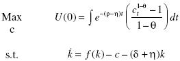
Using Richard's function, it is easy to check that the necessary conditions produce the following dynamical system

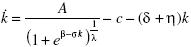
Consumption growth rate is therefore,

There are three solutions. In the first two cases, we have the typical saddle point equilibrium. In the first case (case I), we have the Ramsey model because the marginal productivity of capital is decreasing for all amount of k. In the second case (case II), the marginal productivity of capital is increasing for small quantities of k and deceasing for large values of k.

Case I: A = 100; β = ln3; σ= 2; λ= 3; δ= 0.1; η= 0.025; ρ= 0.05

Case II: A = 100; β =25; σ= 2; λ= 5; δ= 0.1; η= 0.025; ρ= 0.5

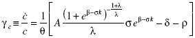
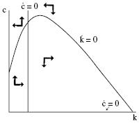
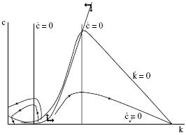
In the last case, as in case III, the marginal productivity of capital is increasing for small values of k and decreasing for large, but now we find that there are two steady states. The first equilibrium, as shown in the graph below, is an unstable equilibrium. The second one is a saddle point. The stable trajectory is shown in the graph for the following parameters.²

Case III: A = 150; β = 25; σ= 0.1; λ= 10; δ= 0.20; η= 0.05; ρ= 0.07

Concluding remark

The inclusion of heterogeneous agents in this framework will be important for future research. Relation between income distribution and growth rates can be explored in this model.

 

Acknowledgments

We thank the financial support provided through the CONACYT Project 82610 from the Mexican Government and C09–FRC–09–10.40 from UASLP.

 

References

Barro, Robert J., Sala–i–Martin Xavier (2004). Economic Growth, New York; Mc Graw Hill.         [ Links ]

Call, Steven and William Holahan (1983). Microeconomía 2^a Edición, Editorial Interamericana.         [ Links ]

Pindyck, Robert and Daniel Rubinfeld (1992). Microeconomics 2nd. Edition, New York: McMillan.         [ Links ]

Ramsey, Frank (1928). "A Mathematical Theory of Saving", Economic Journal, December 1928 No. 38, pp. 543–559.         [ Links ]

Solow, Robert (1956). "A contribution to the theory of Economic Growth", Quarterly Journal of Economics, Vol. 70, pp. 65–94.         [ Links ]

Swan, T. W. (1956). "Economic Growth and Capital Accumulation", Economic Record 32 (November) pp. 334–361.         [ Links ]

 

Nota

² The other trajectories are discarded for violating the optimality conditions.