Artículos

 

Poverty Goals

 

Juan Carlos Chávez–Martín del Campo*

 

Universidad de Guanajuato, UCEA–Campus Marfil, Fracc. I, El Establo, Guanajuato, Gto. 36250, México. Tel: +52(473)735–2925–2925; fax: 52(473)735–2925–2976. E–mail address: *jcc73@quijote.ugto.mx

 

Abstract

We develop a methodology to estimate the required time and the minimum necessary growth rate to meet a poverty goal for a series of counterfactual income distributions and growth scenarios. The methodology can be applied to most poverty measures and is illustrated with data from Madagascar.

Keywords: Poverty goals; poverty measurement; economic growth; Millenium Development Goals; Madagascar.

 

Resumen

Este artículo propone una metodología para estimar el tiempo y la tasa de crecimiento necesarios para alcanzar un objetivo de pobreza, dada una serie de distribuciones del ingreso y escenarios de crecimiento contrafactuales. La metodología se puede aplicar a la mayoría de las medidas de pobreza y es ilustrada con datos de Madagascar.

 

Introduction

Poverty goals are key indicators to evaluate the advancement of development. For instance, in September 2000, the world leaders of the United Nations adopted a document known as the Millenium Declaration which explicitly set an ambitious agenda for international development. It includes a series of goals that are known as the Millenium Development Goals (MDG). The first of them is that the proportion of people living below $1 a day should be halved by 2015, taking the level observed in 1990 as a reference point.¹ Since then, several approaches have been suggested and implemented to study the feasibility of that goal (Besley and Burguess 2003, Deaton 2003, Chen and Ravallion 2004).

This paper develops a simple methodology to estimate two parameters of interest for the analysis of poverty goals: the required time and the minimum necessary growth rate to meet a poverty goal under several growth and distribution scenarios.²

The methodology has several advantages. First, it can be applied to practically all poverty measures used in applied work. Second, it takes into account country heterogeneity: the parameters of interest can be estimated in a case by case basis, instead of estimating a cross–country regression. As noticed by Bourguignon (2002), this approach is more appropriate since both the development and inequality level of a country do affect the growth elasticity of poverty reduction. Third, the parameters can be estimated from aggregate data. Finally, we do not need a panel or a cross section of countries to obtain our estimators.

We applied the methodology to Madagascar, one of the poorest countries in the world. In this country, poverty has increased and deepened substantially over the last two and a half decades, with real per capita income having decreased by 40 percent between 1971 and 1991. Given this economic scenario, meeting the MDG in Madagascar is really challenging and, therefore, analyzing the feasibility of halving poverty by 2015 is of paramount importance.

The following section describes the methodology. Section 3 introduces inequality into the analysis. Section 4 illustrates the methodology using data from Madagascar. Section 5 concludes.

 

Methodology

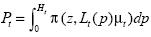
Let F_t (y) be the income distribution and y_t (p) be the p quantile of that distribution at time t. We focus on poverty measures that can be fully characterized in a general form as follows

(1)

P₁= P(µ, z, L_t)

where µ_t, is the mean income, z is the poverty line, and L_t is the Lorenz curve.

As a special case for this class of measures, we have the family of additively separable poverty measures, which can be written as

(2)

where π (·) is the poverty evaluation function and H_t is the proportion of people whose incomes are below the poverty line, z.³ For instance, the Foster–Greer–Thorbecke (1984) family of poverty measures is

(3)

As α gets larger, the P_α measure get more sensitive to extremely low incomes. In fact, for some values of α , the P_α measure satisfies two axioms that an "ethical" measure of poverty should satisfy (Sen 1976):

Monotonicity Axiom: Ceteris paribus, a reduced income for a poor person should result in an increase in the poverty measure.

Transfer Axiom: Ceteris paribus, a pure income transfer from a poorer to a richer person should increase the poverty measure.

Foster et. al., (1984) showed that for α >0, P_α satisfies the monotonicity axiom and for α >1, P_α satisfies the transfer axiom.

Let P^* be a poverty goal. The needed mean income, µ^*, to meet this poverty goal for a given income distribution, , and an exogenous poverty line, z, is defined as

(4)

µ^* = inf {µ : P(µ, z, ) ≤ P^*}

Notice that the time taken to meet the poverty goal, P^*, given , , z, and an annual per capita growth rate, , is implicitly given by . By reordering this equating, we get

(5)

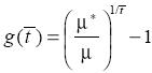
Analogously, the minimum necessary growth rate, g (), to meet the poverty goal, P^*, in years, holding both the income distribution and the poverty line constant, is

(6)

 

Incorporating Inequality into the Analysis

Although most of the poverty changes are explained by growth in average incomes (Kraay 2006), changes in income inequality may play an important role in meeting poverty goals in the medium–to–long run, particularly in very unequal societies. There is a problem, however, when trying to incorporate changes in inequality into the analysis because inequality in income distribution can change in an infinite number of ways.

To handle this problem, we use the lognormal distribution to approximate the distribution of income. This parameterization is very standard in applied work for its tractability and generally fits the data very well (Lopez and Serve, 2006). Exploiting the one to one mapping that arises under lognormality between the Lorenz curve and the Gini coefficient, G , and using the fact that L_t (p) = Φ(Φ)^–1(p) –σ_t) (Aitchison and Brown), from (2) it can be shown that

(7)

where

(8)

and

(9)

where Φ(·) and Φ(·) are, respectively, the cumulative distribution function and the probability density function for the standard normal. Particularly, the head count ratio can be reformulated as

(10)

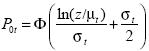
It can be easily shown that . Therefore, for a given G we have a unique average income, µ^*(G), that solves

(11)

P₀ (µ, z, G) = P^*

From this equation, we can estimate the parameters of interest, t () and g (), for counterfactual income distributions.

 

Meeting the Millenium Development Goals in Madagascar

To illustrate the methodology developed in this paper, we focus on the first of the MDG for Madagascar. We go beyond the estimation of the parameters of interest for P₀ by also estimating them for the poverty gap, P₁, and its square, P₂.

For the estimation of the parameters of the Lorenz curve, we follow Datt and Ravallion (1992) in using two specific parameterizations: the General Cuadratic Lorenz curve (Villasenor and Arnold 1989) and the Beta Lorenz curve (Kakwani 1980). Applying their methodology, we are able to find µ^*for the P_α family of poverty measures.⁴ The rest of the calculations are simple substitutions into equations (5) and (6).

To estimate the parameter of the Lorenz curve, we have made use of PovcalNet⁵, a website developed by the World Bank Research Department that provides interactive computational tools that allow one to estimate the parameters of the Lorenz curve for the two parameterizations mentioned above for a series of countries. In the case of Madagascar, the Cuadratic Lorenz curve is used in the estimation of µ^*.⁶ For this application, initial average income and income distribution are obtained from the 2001 data set, the most recent data for Madagascar available at PovcalNet. For that particular year, average income was $4028. a month in 1993 PPP dollars and the Gini coefficient was 0.48.

From table 1, it is clear that Madagascar must register annual growth rates of at least 8% to meet the MDG. Halving the poverty gap, P₁, demands a similar growth rate (7%). Meeting the goal of halving the squared poverty gap is even more ambitious: the growth rate must be at least 15% per year to halve P₂ . Table 1 also presents the required time to meet the different poverty goals under several growth scenarios. Even under an optimistic scenario with an annual growth rate of 3%, it would take over 35 years to halve the proportion of poor people. Given Madagascar's poor economic performance between 1990 and 2004⁷, meeting the MDG would not appear to be feasible under the conditions observed during that period.

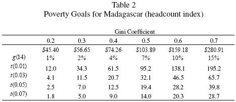
We also explore the effects of changes in inequality on the parameters of interest. As already mentioned in section 3, we assume lognormality to get a one to one mapping between the headcount ratio and the Gini coefficient. We simulate a zero economic growth scenario between 2001 and 2015 to obtain the order of magnitude in the reduction of inequality required to meet the first of the MDG. The Gini coefficient would need to decline from 0.48 to 0.14 to halve the proportion of people living in extreme poverty if Madagascar's economy were stagnant. An alternative analysis would simulate the parameters of interest for several counter–factual income distributions. These results are reported in table 2. The first row provides the required mean income, µ^*(G), for several levels of inequality. As expected, µ^*(G) is increasing on the Gini coefficient. The second row reports the minimum necessary annual growth rate between 2001 and 2015 to meet the first of the MDG. The remaining rows present the required time to meet the goal for several combinations of growth rates and Gini coefficients. This makes it possible to get an idea of what could happen if inequality rises or decreases in the future. For instance, if the Gini coefficient reduces from 0.5 to 0.4, the minimum necessary growth rate decreases to 4 percent, almost half the required growth rate when G =. 05.

 

Conclusions

The estimation of the required time and the minimum necessary growth rate under alternative distributional and growth scenarios can shed some light on the feasibility of a poverty goal. Moreover, it can help to identify the necessity of implementing policies and reforms oriented toward pro–poor growth when current economic and institutional conditions do not generate a propitious environment to meet a previously set poverty goal. As noticed by Besley and Burgess (2003), the institutional and political context in which policy and accumulation decisions are taken are of paramount importance for improving the quality of growth in the sense of making it more pro–poor.

 

References

Aitchison, J. and J. Brown (1966). The Lognormal Distribution, Cambridge University Press.         [ Links ]

Besley, Timothy and Robin Burgess (2003). "Halving global poverty", Journal of Economic Perspectives 17(3), 3–22.         [ Links ]

Bourguignon, Francois (2002). "The growth elasticity of poverty reduction : explaining heterogeneity across countries and time periods", Technical report.         [ Links ]

Chen, Shaohua and Martin Ravallion (2004). "How have the world's poorest fared since the early 1980s?", Policy Research Working Paper Series 3341, The World Bank.         [ Links ]

Datt, Gaurav (1998). "Computational tools for poverty measurement and analysis", Technical report.         [ Links ]

Datt, Gaurav and Martin Ravallion (1992). "Growth and redistribution components of changes in poverty measures : A decomposition with applications to Brazil and India in the 1980s", Journal of Development Economics 38(2), 275–295.         [ Links ]

Deaton, Angus (2003). "How to monitor poverty for the millenium development goals", Journal of Human Development 4(3), 353–378.         [ Links ]

Foster, James, Joel Greer and Erik Thorbecke (1984). "A class of decomposable poverty measures", Econométrica 52(3), 761–66.         [ Links ]

Gastwirfh, Joseph L. (1971). "A general definition of the lorenz curve", Econométrica 39(6), 1037–39.         [ Links ]

Kakwani, Nanak (1980). "On a class of poverty measures", Econométrica 48(2), 437–46.         [ Links ]

Kraay, Aart (2006). "When is growth pro–poor? evidence from a panel of countries", Journal of Development Economics 80(1), 198–227.         [ Links ]

Li, Hongyi, Lyn Squire and Hengfu Zou (1998). "Explaining international and intertemporal variations in income inequality", Economic Journal 108(446), 26–43.         [ Links ]

Lopez, Humberto and Luis Serven (2006). "A normal relationship? poverty, growth, and inequality", Policy Research Working Paper Series 3814, The World Bank.         [ Links ]

Ravallion, Martin (2001). "Growth, inequality and poverty: Looking beyond averages", World Development 29(11), 1803–1815.         [ Links ]

Sen, A. (1976). 'Poverty: An Ordinal Approach to Measurement', Econométrica 44, 219–231.         [ Links ]

Villasenor, Jose A. and Barry C. Arnold (1989). "Elliptical lorenz curves", Journal of Econometrics 40(2), 327–338.         [ Links ]

World Bank (2006). World Development Indicators 2006, World Bank Publications.         [ Links ]

 

Notes

¹ For a more complete description of the goals see www.developmentgoals.org.

² The relative importance of both growth and inequality for poverty is well documented (Datt and Ravallion 1992, Li, Squire and Zow 1998, Ravallion 2001).

³ To obtain this expression we have used the fact that L'(p) µ =F^–1(p) (Gatswirth 1971).

⁴ See Datt(1986) for details.

⁵ http://iresearch.worldbank.org/PovcalNet/.

⁶ L (p; π) represents a valid Lorenz curve if and only if L (0, π) = 0, L (1, π) = 1, L' (0⁺, π) = ≥ 0, and L' (p, π) ≥ 0 in . In the case of Madagascar, these conditions are satisfied for the Cuadratic Lorenz curve.

⁷ The annual per capita growth rate was –1.1% (World Bank 2006).