


Serviços Personalizados
Journal
Artigo
 texto em
  Inglês (pdf)
 Artigo em XML
 Referências do artigo
 Enviar este artigo por email
Indicadores
-
 Citado por SciELO
 -
 Acessos
Links relacionados
-
 Similares em
SciELO
Similares em
SciELO
Compartilhar

 Permalink
Agricultura, sociedad y desarrollo
versão impressa ISSN 1870-5472
agric. soc. desarro vol.15 no.3 Texcoco Jul./Set. 2018
Articles
Factors that Determine the Maize Production Yields in Mexico: Evidence from the 2007 Agriculture and Livestock Census
1Banco de México. Av. 5 de Mayo No. 18, Col. Centro, México, CDMX. (shcadet@banxico.org.mx)
2Dirección Nacional de Medio Ambiente. Galicia 1133, Montevideo, Uruguay. (sguerreroe@gmail.com)
This article presents a description of the evolution of the maize production yields in Mexico. It is compared with the evolution of yields in other producer countries and the main factors that define the maize yields are derived, through an econometric analysis. This analysis is carried out with data from the 2007 Agriculture and Livestock census at the level of municipality of the economic units that reported producing maize and consists of a linear estimation with crossed-section data of the yields in economic units as function of technological, credit, socioeconomic, geographic and climate variables, controlling for dummies of productive cycle and state. The results point to the use of improved seeds, insecticides, access to credit and irrigation as the variables that have highest correlation with the yields in maize production in Mexico.
Key words: credit; maize yields; irrigation; improved seed
En este artículo se hace una descripción de la evolución de los rendimientos de la producción de maíz en México. Se compara con la evolución de los rendimientos en otros países productores y se derivan los principales factores que determinan los rendimientos de maíz, a través de un análisis econométrico. Dicho análisis se realiza con datos del Censo Agropecuario 2007 a nivel de municipio de las unidades económicas que reportaron producir maíz y consiste en una estimación lineal con datos de sección cruzada de los rendimientos de las unidades económicas como función de variables tecnológicas, crediticias, socioeconómicas, geográficas y climáticas, controlando por dummies de ciclo productivo y entidad federativa. Los resultados apuntan a que el uso de semillas mejoradas, insecticidas, el acceso al crédito y el riego son las variables que tienen una mayor correlación con los rendimientos de la producción de maíz en México.
Palabras clave: crédito; rendimientos del maíz; riego; semilla mejorada
Introduction
In general, not only in Pre-Hispanic times but also until the middle of the 20th century, the processes of improvement of maize seed with which the yields were increased were long term3. This trend was modified since 1960, where in a period of 25 years the global agricultural yields doubled (Hazell, 2009).
This increase in the yields is explained by the “Green Revolution”, process that began in the decade of the 1970s, driven because some developing countries experienced famines and increases in malnutrition (Hazell, 2009), which led the Rockefeller and Ford foundations to promote a program of research and development of agricultural technologies focused on increasing the wheat, rice and maize yields, primarily. The development of new varieties of wheat, rice and maize generated by investments in agricultural research mentioned, in addition to the more generalized application of fertilizers, insecticides, machinery and credit to acquire inputs, is known as the “Green Revolution” (Borlaug, 1972)4.
Although a great part of the development of cultivation technologies in the Green Revolution were carried out in Mexico, the country’s yields remained laggard with regards to other countries. Table 1 compares the average yields per decade between Mexico and other countries and regions of the world. It shows that in the 1960s the countries of the European Union and the United States of North America had yields higher than two tons per hectare in grain cultivation, while various developing countries, including Mexico, did not manage to achieve this figure5. It wasn’t only Mexico that was not able to increase its yields in the decade of the 1970s; in the 2000s it had lower average yield than other relevant developing countries in grain production, such as China, Brazil and Argentina.
Table 1 Average maize yields per period.
| Cifras en toneladas por hectárea | |||||
| 1961-1969 | 1970-1979 | 1980-1989 | 1990-1999 | 2000-2012 | |
| EE. UU. | 4.5 | 5.6 | 6.6 | 7.7 | 9.2 |
| México | 1.1 | 1.3 | 1.8 | 2.3 | 3.0 |
| Unión Europea | 2.6 | 3.9 | 5.2 | 5.7 | 6.6 |
| Mundo | 2.2 | 2.8 | 3.4 | 4.0 | 4.8 |
| China | 1.6 | 2.4 | 3.6 | 4.8 | 5.2 |
| India | 1.0 | 1.1 | 1.3 | 1.6 | 2.1 |
| Brasil | 1.3 | 1.5 | 1.8 | 2.4 | 3.7 |
| Argentina | 1.9 | 2.7 | 3.3 | 4.5 | 6.5 |
Source: authors’ elaboration based on the data from the Statistics Division of the FAO (FAOSTAT).
This article has the main objective of trying to shed light on different factors, both technological and of agriculture and livestock policy that may be correlated with maize yields in Mexico in 2007. With this, we attempt to inform public policy makers about the factors that define to a large extent the maize yields.
In the literature there are various studies that attempt to measure, by way of econometric models, the impact of climate, socioeconomic and technological variables for the United States (Kaufmann and Snell, 1997) or to measure potential impacts of climate change on agricultural yields in the United States (Schlenker and Roberts, 2006) and in Mexico (Olivera, 2013). However, for Mexico there are no studies available that directly relate the impact of various technological variables and agriculture and livestock policies on maize yields. In this study an econometric exercise is performed that is similar to the one carried out by Kaufmann and Snell (1997), through which the average yields per municipality are estimated as a function of technological, geographic and socioeconomic variables, using data from the Agriculture and Livestock Census 2007. The econometric model used does not attempt to establish causal relations, but rather to show correlations between diverse variables and the average yields of the economic units in each municipality of the country. Additionally, the economic and technological processes that influenced historically the evolution of the yields in maize production are contextualized, both in Mexico and in other developing nations that produce maize.
The results point to the fact that variables which associate positively with the yields are primarily those of technological nature and access to credit. In particular, those productive units that report having used improved seed6, having a credit, or having used insecticides report higher yields: an increase of 10 % in the use or access of those variables is correlated with an increase in the yield of the crop in 0.35, 0.31 and 0.25 tons per hectare, respectively, which would represent an increase of 12.2 %, 10.8 % and 8.7 % in the average domestic yield. In terms of credit, investment credit is the one with highest level of association with yields, which is used to finance the acquisition of fixed assets. Finally, no important effects were found from the use of fertilizers or in the Program of Direct Supports to the Farmland (Programa de Apoyos Directos al Campo, PROCAMPO).
The article is organized in the following way: Section 1 argues the evolution of the maize yields in various producing nations, including Mexico, emphasizing the agriculture and livestock policies that had an impact on them; Section 2 shows a literature review on the subject; Section 3 specifies the data and the econometric method; Section 4 discusses the results; and Section 5 presents the conclusions.
Maize yields in emerging nations
Maize yields in developing countries
Since 1960, the differences in the trajectories of maize yields that different countries have followed respond to socioeconomic and geographic factors. In China, the average yield in the 1980s exceeded the three tons per hectare (Table 1), which was associated to the changes in agrarian and technological policies. In this decade, the system of communes in effect since 1950 was replaced by the system of family responsibility, with which the peasant in family farms produced and sold his harvest to the state through contracts (McMillan et al., 1989; Fan, 1991; Lin, 1992; Salvador, 2008). Additionally, research institutes were allowed to self-finance through the sale of applied technology (Pray et al., 1997), with which agricultural research was fostered and highly productive agronomic systems were established thanks to irrigation (Wang, 2000). This allowed for China to become global leader in agrarian biotechnology by the end of the 1990s, being one of the countries with highest investment in rural research and development in the world (Huang and Rozelle, 2009).
In Argentina, since the decade of the 1990s a structural change of the agricultural sector took place, due to the technological advancement, the emergence of new forms of organization between producers and suppliers, and to the changes in economic and fiscal policy, with which it was managed to obtain maize yields of more than four tons per hectare (Table 1). The “sowing pools” arose as new forms of organization that attained agreements for producers to be in charge of performing farming tasks, while the suppliers granted technical resources, financing and transport, with the aim of generating scale economies and high yields, allowing for earnings to be distributed at the end of the harvest (World Bank, 2006; Sturzenegger and Salazni, 2007; Lence, 2010).
The increase in maize yields in Argentina was due to diverse factors such as investment in research and development by transnational agrichemical companies, as well as the increase in use of fertilizers, the incorporation of supplementary irrigation, and the renovation of machinery and equipment, culminating with the adoption of transgenic seeds since the 1998/1999 cycle (Gear, 2006; Gutman and Lavarello, 2007). This was possible, to a large extent, because of the free trade policy that reduced the imports tariffs on inputs and fixed assets, which, in turn, allowed a greater flexibility in the commercialization of the crops (Lence, 2010).
In Brazil, the significant changes in yields began since the 1990s, decade when the trade policy allowed greater access to international markets, during which strong investments were made on infrastructure and agricultural research and a strengthening of the private sector in the agriculture and livestock sector (Rosegrant et al., 2006). Also in the 1990s, improvements took place in the yields of different crops derived from the research and development that EMBRAPA (Empresa Brasileira de Pesquisa Agropecuaria) fostered, institute in charge of agricultural research, both in local and state institutions. This drive allowed for research centers to have a national presence and to develop new varieties of seeds of various crops, among them, maize (Magalhaes and Diao, 2009).
In 2008/2009, approximately ten years after the Argentinian case, the sowing of transgenic maize was approved, which led to an increase in the yields’ trend, as had happened in Argentina (Parentoni et al., 2013).
In sum, the increases in maize yields in the main developing countries are linked to: 1) trade policies, with which there was access to external markets, both to export and to import inputs; 2) research and development applied to agriculture, as well as the adoption of transgenic seeds; and 3) strengthening of commercial chains, coordinated by the state in the case of China and promoted privately in the case of Argentina and Brazil.
Maize yields in Mexico
Maize is a crop native to Mexico. The first vestiges of the plant, called teocintle, were found in Tehuacán, Puebla, and have an age of between 4500 and 7000 years (McClung de Tapia, 1997). The creation of maize varieties with higher yields, more resistant and apt to be sown in different climates was a process that took Pre-Hispanic peoples thousands of years. This process involved seed selection, sowing techniques, and its cultivation in different climates (Benz, 1997). Presently, there are more than forty maize races and hundreds of varieties.
In Mexico, in the 1970s and beginning of the 1980s, the state was the promoter of agricultural and livestock activity, so that institutions were created in favor of agricultural producers that had government infrastructure which carried out stockpiling, storage, commercialization and distribution of grains; likewise, there were large subsidies both to producers and to consumers of maize and its byproducts. Facing climate fluctuations and the scarce transfer of technology, guarantee prices arose to foster production, which increased in a relevant way the public expenditure, which is why at the end of the 1980s and in the decade of the 1990s, economic and constitutional reforms were implemented that liberalized various sectors of the economy, among them the agriculture and livestock sector, with which the government ceased to play a prominent role in the commercialization of agricultural and livestock products, the guarantee prices were eliminated, and the subsidies were dissociated (Appendini, 2005).
In Mexico, the trade policies that liberalized the maize market with the entry of NAFTA in 1994 do not seem to have generated an important increase in the average of maize yields at the national level (Figure 1).
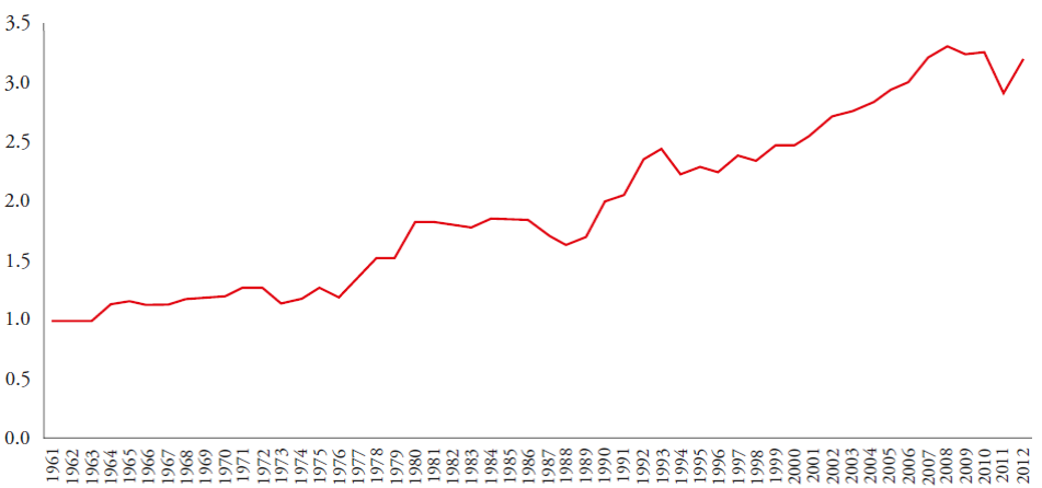
Source: Authors’ elaboration based on data from FAO’s Statistics Division (FAOSTAT).
Figure 1 Mexico: Maize yields from 1961 to 2012. Figures in tons per hectare.
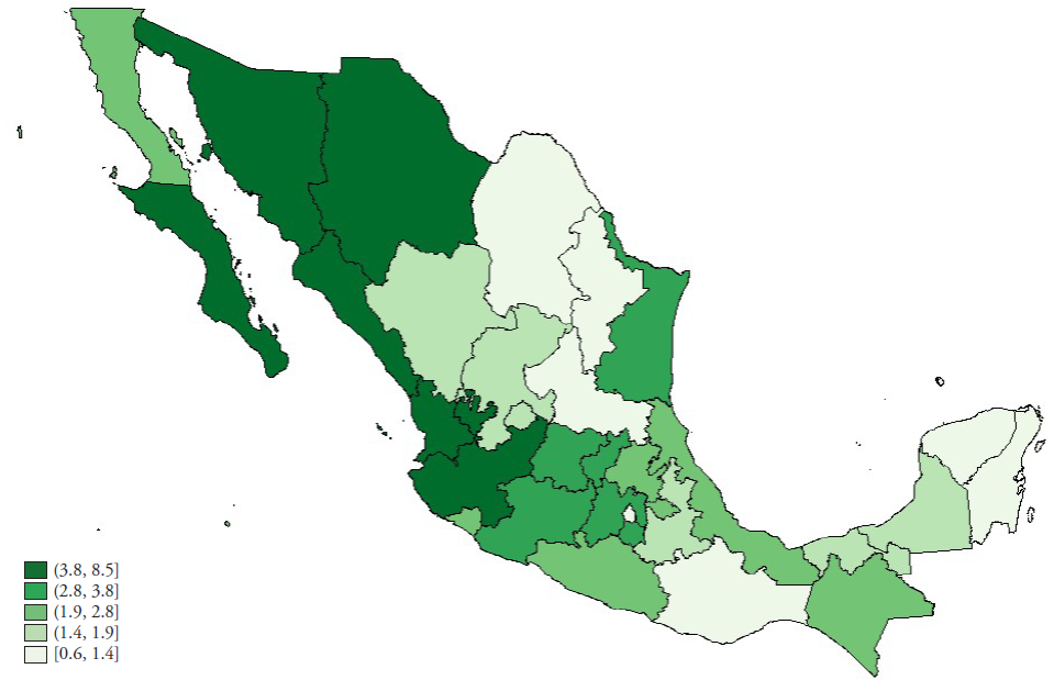
However, there is great heterogeneity in the yields at the regional level, where the highest yields were concentrated in the Northeast and Bajío regions of the country, situation that contrasts with the Center and South regions, where in some states the average yields did not exceed the three tons per hectare in the period between 2000 and 2010 (Figure 2).
According to data from the Agriculture and Livestock Census 2007, published by the National Institute of Statistics and Geography (Instituto Nacional de Estadística y Geografía, INEGI), there are more than two million producers devoted to maize cultivation. It is important to mention that it was the last census that INEGI performed up until this study, while the previous Agriculture and Livestock Census was in 1991.
According to data from the Agrifood and Fishing Information Service (Servicio de Información Agroalimentaria y Pesquera, SIAP)7 and the Statistics Division from the Food and Agriculture Organization of the United Nations (FAO)8, currently, the most common maize varieties sown in Mexico are white and yellow. In 2010, 23.3 million tons of maize were produced in Mexico, of which approximately 91.0 % corresponded to the white maize variety and the rest to the yellow. This allowed Mexico to be the fourth maize producer, after the United States, China and Brazil, globally, with a participation of 2.8 % in that year.
The differences at the regional level can be explained in part by the new instruments for promotion of agricultural and livestock production and trade that were created starting in 1994, such as PROCAMPO, and the programs for support to commercialization operated by Supports and Services to Agriculture and Livestock Commercialization (Apoyos y Servicios a la Comercialización Agropecuaria, ASERCA), which is currently a decentralized administrative organization of the Ministry of Agriculture, Livestock Production, Rural Development, Fishing and Food (Secretaría de Agricultura, Ganadería, Desarrollo Rural, Pesca y Alimentación, SAGARPA). These new policies allowed for capitalized producers to be organized according to the openness and promotion of ejido privatization, controlling the market and trading their harvests directly, thanks to their competitive abilities, complementary supports, and backing by ASERCA; the large-scale producers located in the Northwest and Bajío regions of the country were especially favored (Aguilar, 2004). In particular, an important growth took place in maize yields of the irrigation zones where commercial producers were concentrated, which differed from the yields in the rainfed zones that did not exceed the two tons per hectare during the first decade of the 21st century, and which concentrated the small-scale or subsistence producers (Yunez and Serrano, 2010).
Literature review
Various previous studies have focused on understanding the determinants of maize yields. Evenson and Kislev (1973) found a strong and persistent relation between agricultural research and maize yields, with a sample of 49 producing countries. Gowon et al. (1978) analyzed the response of yields in California, Colorado and Utah, states of the American Union, in face of factors such as irrigation under a specific type of soil and whose results differed, depending on the phenological stages of the crop. Other more recent studies (Kaylen et al., 1992; Schlenker and Roberts, 2006; Roberts et al., 2012) incorporated agronomic knowledge to climate variables such as temperature and precipitation to relate them econometrically with the yields and, in the case of the last two studies, to project the possible impact of climate change on maize yields in the United States.
In their turn, Kaufmann and Snell (1997) estimated a model for maize yields in the municipalities of the United States, incorporating socioeconomic determinants such as market conditions, production scales, technology adoption and public policies, as well as climate variables. Ruttan (2002) performed a detailed analysis of the technical, institutional and resource restrictions for the growth of agricultural productivity in the last 50 years of the 20th century, where he concluded that most of the developing countries should invest more in agricultural research and development, technical training and infrastructure to increase the yields in this century. Kamruzzaman et al. (2000) examined the effect of credit on the yields and on the technical efficiency of rice production in the district of Comilla, Bangladesh, and found that the producers who have credit have a higher yield potential than those who do not, concluding that credit has a positive impact to increase the technical efficiency of producers.
The effects of climate change have also been studied through regressions of the yields at the level of municipality in climate variables. Olivera (2013) finds that climate change will have negative effects on maize yields in Mexico, especially in rainfed zones. Likewise, Galindo (2009) indicates that the impacts on the yields derived from climate change will be heterogeneous by regions and each productive cycle will have different response sensitivities to temperature and precipitation in Mexico.
Materials and Methods
Data
Derived from the literature review, it was determined that the factors that could impact a sustained increase in maize yields in Mexico would be those related to the production (infrastructure, biotechnology, use of agrichemicals, and use of credit), geography, climate, agriculture and livestock policies, and socioeconomic factors.
Therefore, the following data were obtained, relative to the use of chemical fertilizers, improved seed, insecticides, tractor, natural fertilizer, controlled burning, credit, as well as the scale and schooling, aggregated at the municipal level for the cultivation of maize grain, from the Agriculture, Livestock and Forest Census 2007, provided by INEGI, which were requested from that organization to carry out this study. The irrigation variable was obtained from the data of the irrigation surface from 2005 of the Agrifood Information System for Consult (Sistema de Información Agroalimentaria de Consulta, SIACON) of the SAGARPA.
The socioeconomic variables of total population, availability of public services and population recipient of public health services, were obtained from the Population and Housing Census 2005 elaborated by INEGI. These were included to get a better coverage of possible variables that could influence the maize yields, through their indirect incidence on the labor market. For example, Barbier and Burgess (1996) find a positive relation between the population and the agricultural surface sown in Mexico, which impacts directly the agricultural yields. López-Feldman (2012) estimates a positive relation between the marginalization index of the municipalities in Mexico, and the expansion of the agricultural frontier. In turn, Deininger and Minten (1999) find a negative relation between poverty and agricultural land use in Mexico.
Likewise, the price of maize was included, which represents the average of the price between 2006 and 2007 per municipality. The variable Amount of PROCAMPO per producer at the municipal level was obtained from the Municipal System of Databases (Sistema Municipal de Bases de Datos, SIMBAD) of the INEGI for the years of the Census and represents the average amount of transferences performed to producers by PROCAMPO in each municipality.
Geographic data were also obtained, such as distance to the closest city, density of roads, distance to the coast, length of the road, and slope of the land from the geospatial data of Use of Land and Vegetation from INEGI. These variables have an impact on the surface sown and on the conversion of land use (Barbier and Burgess, 1996).
Similarly, the characteristics of the land per municipality were incorporated, using the geospatial soil data elaborated by the National Institute of Forest, Agriculture and Livestock Research (Instituto Nacional de Investigaciones Forestales Agrícolas y Pecuarias, INIFAP) and the National Commission for the Knowledge and Use of Biodiversity (Comisión Nacional para el Conocimiento y Uso de la Biodiversidad, CONABIO) from 1995. These characteristics were classified per type of soil, physical composition and texture. There are 21 types of soil, six categories for the physical composition and three for texture.
Finally, in the case of the climate variables, the data of accumulated precipitation and average growing degree days (GDD), of the years 2003 to 2007 per municipality present during the growth stage of maize, were included. The data concerning the precipitation and temperature at the level of meteorological station were provided by the National Meteorological Service and processed by the authors to obtain data at the municipal level in agricultural zones.
The growing degree days are used to capture the exposure to heat during the cultivation in the growth stage, which is why with the data of temperature the calculation was carried out in the following way (Roberts et al., 2012):
min{(Th+Tl) /2 ,Tm}-Tb
where Th is the maximum temperature, Tl the minimum temperature, and Tb the base temperature (10 °C) and Tm the upper limit (30 °C).
Tables 2a and 2b from the Annex show the descriptive statistics of the main variables. Table 2a present averages per municipality for all the variables used in this study and Table 2b presents the averages at the national level. It is done this way because there are important variations in terms of the degree of use of some inputs in maize production, whether if measured as proportion of the national surface or as average of the municipal surface. As can be observed, the penetration of improved seed is 12 % in average in the municipalities (Table 2a), but measured in terms of the total surface sown with maize in the country (Table 2b) represents 18 %, figure close to that reported by other studies9.
Table 2a Descriptive statistics of averages per municipality.
| Variables | Observaciones | Media | Desviación Estándar | Mínimo | Máximo |
| Rendimientos (tonelada por hectárea) | 1913 | 2.86 | 2.12 | 0.17 | 13.17 |
| Irrigación (porcentaje de superficie de riego) | 1913 | 0.24 | 0.36 | 0.00 | 1.00 |
| Fertilizantes Químicos (porcentaje de fertilizantes químicos aplicados en superficie agrícola) | 1913 | 0.32 | 0.28 | 0.00 | 1.00 |
| Semilla mejorada (porcentaje de semilla mejorada aplicada en superficie agrícola) | 1913 | 0.12 | 0.19 | 0.00 | 1.00 |
| Insecticidas (porcentaje de insecticidas aplicados en superficie agrícola) | 1913 | 0.12 | 0.18 | 0.00 | 0.91 |
| Uso de tractor (porcentaje de unidades de producción que usan tractor) | 1913 | 0.55 | 0.32 | 0.00 | 1.00 |
| Abono natural (porcentaje de abono natural aplicado en superficie agrícola) | 1913 | 0.07 | 0.11 | 0.00 | 0.88 |
| Quema controlada (porcentaje de quema controlada aplicada en superficie agrícola) | 1913 | 0.02 | 0.04 | 0.00 | 0.80 |
| Uso de crédito (porcentaje de unidades de producción que cuentan con crédito) | 1913 | 0.05 | 0.08 | 0.00 | 1.00 |
| Uso de crédito de avío (porcentaje de unidades de producción que cuentan con crédito de avío) | 526 | 0.06 | 0.11 | 0.00 | 0.66 |
| Uso de crédito refaccionario (porcentaje de unidades de producción que cuentan con crédito refaccionario) | 526 | 0.01 | 0.01 | 0.00 | 0.16 |
| Uso de otro tipo de crédito (porcentaje de unidades de producción que cuentan con otro tipo de crédito) | 526 | 0.02 | 0.02 | 0.00 | 0.31 |
| Escala mayor a cinco hectáreas (porcentaje de unidades de producción que cuentan con más de cinco hectáreas) | 1913 | 0.40 | 0.28 | 0.00 | 1.00 |
| Escala mayor a cinco hectáreas al cuadrado (porcentaje de unidades de producción que cuentan con más de cinco hectáreas, elevado al cuadrado) | 1913 | 0.24 | 0.28 | 0.00 | 1.00 |
| Superficie sembrada de maíz blanco (cifras en porcentaje) | 1890 | 0.97 | 0.12 | 0.00 | 1.00 |
| Capacitación(porcentaje de unidades de producción que contaron con capacitación) | 486 | 0.03 | 0.05 | 0.00 | 0.42 |
| Densidad de las carreteras (longitud/área) | 1913 | 1.46 | 1.08 | 0.00 | 12.14 |
| Distancia a la ciudad más cercana >500 (km) | 1913 | 150.52 | 90.11 | 3.72 | 486.99 |
| Distancia a la costa (km) | 1913 | 144.17 | 101.77 | 0.22 | 611.25 |
| Longitud de la carretera (miles de km.) | 1913 | 0.08 | 0.10 | 0.00 | 1.16 |
| Pendiente del suelo | 1913 | 5.69 | 3.85 | 0.06 | 19.52 |
| Población con algún año de escolaridad (cifras en porcentaje) | 1913 | 0.74 | 0.13 | 0.27 | 1.00 |
| Población total (millones de habitantes) | 1913 | 0.04 | 0.10 | 0.00 | 1.49 |
| Población con acceso a servicios públicos: agua, red pública, drenaje y energía eléctrica (cifras en porcentaje) | 1913 | 0.59 | 0.25 | 0.00 | 0.96 |
| Población derechohabiente a servicios de salud (cifras en porcentaje) | 1913 | 0.31 | 0.21 | 0.00 | 0.86 |
| Monto PROCAMPO por productor (miles de pesos) | 1885 | 4.94 | 4.54 | 0.50 | 38.03 |
| Precio medio rural del maíz (cifras en pesos por tonelada) | 1890 | 2528.75 | 537.55 | 1092.59 | 4202.13 |
Table 2b Descriptive statistics as averages at the national level.
| Variables | PV | OI | Ambos ciclos |
|---|---|---|---|
| Fertilizantes químicos (porcentaje de fertilizantes químicos aplicados en superficie agrícola) | 39.7 | 31.1 | 38.6 |
| Semilla mejorada (porcentaje de semilla mejorada aplicada en superficie agrícola) | 17.5 | 23.2 | 18.3 |
| Insecticidas (porcentaje de insecticidas aplicados en superficie agrícola) | 16.5 | 22.1 | 17.2 |
| Uso de tractor (porcentaje de unidades de producción que usan tractor) | 39.8 | 36.7 | 39.6 |
| Abono natural (porcentaje de abono natural aplicado en superficie agrícola) | 6.9 | 3.4 | 6.5 |
| Quema controlada (porcentaje de quema controlada aplicada en superficie agrícola) | 2.2 | 1.5 | 2.1 |
| Uso de crédito (porcentaje de unidades de producción que cuentan con crédito) | 3.1 | 8.4 | 3.4 |
| Uso de crédito de avío (porcentaje de unidades de producción con crédito de avío) | 1.8 | 6.9 | 2.1 |
| Uso de crédito refaccionario (porcentaje de unidades de producción con crédito refaccionario) | 0.3 | 0.3 | 0.3 |
| Uso de otro tipo de crédito (porcentaje de unidades de producción con otro tipo de crédito) | 0.8 | 1.0 | 0.8 |
| Capacitación (porcentaje de unidades de producción que contaron con capacitación) | 2.2 | 4.7 | 2.4 |
Empirical model
The econometric estimation of the yields as function of the variables specified in the previous subsection is detailed in this section. Three specifications of the model are performed: 1) controlled for technological and credit variables; 2) geographic, climate and access to infrastructure data are added; and 3) socioeconomic variables are included. The model is based on Kaufmann and Snell (1997), and it is expressed in the following way:
where Rend indicates yields (tons of maize per hectare), c represents the cycle (Spring-Summer or Fall-Winter), and m the municipality; Tech represents the set of technology variables like use of improved seed, irrigation, fertilizers, insecticides, controlled burning, natural fertilizer, use of tractor, scale, credit and surface sown with white maize; Geog denotes the set of controls for geographic characteristics such as distance to cities, average slope, distance to the coast and type of soil, as well as precipitation and growing degree days (GDD). Finally, the vector Socio contains socioeconomic variables such as schooling, total population, availability of public services, population that has access to public health services, average amount of PROCAMPO assigned per producer and mean rural maize price.
Each specification is estimated for three cases: using the units that sow in the spring-summer cycle (PV), fall-winter (OI), and in both cycles. In the three cycles it is controlled for dummies of federal state µ e and, additionally, in the third cycle it is controlled for sowing cycle µ c .
Results and Discussion
In the case of the Spring-Summer cycle (Table 3a), the statistically significant factors with greatest impact are the use of improved seed, credit and insecticides, and with lower impact, although still significant when there is irrigation and use of natural fertilizer. In the fall-winter cycle (Table 3b) it can be seen that the impacts are lower than in the spring-summer cycle, but the relevance of the use of improved seed, insecticides and natural fertilizer, is repeated, not coinciding in that for this cycle the use of fertilizers is significant.
Table 3a Results- PV Cycle.
| Variables | 1 | 2 | 3 | |||
|---|---|---|---|---|---|---|
| Irrigación | 1.7554 | *** | 1.4529 | *** | 1.4531 | *** |
| (0.3413) | (0.3045) | (0.3245) | ||||
| Fertilizantes químicos | -0.1647 | -0.1546 | -0.1631 | |||
| (0.2277) | (0.2351) | (0.2447) | ||||
| Semilla mejorada | 3.9659 | *** | 4.0994 | *** | 4.0146 | *** |
| (0.3852) | (0.3762) | (0.419) | ||||
| Insecticidas | 2.7507 | *** | 2.5019 | *** | 2.5671 | *** |
| (0.5751) | (0.633) | (0.661) | ||||
| Uso de tractor | 0.3010 | 0.3235 | 0.2240 | |||
| (0.1879) | (0.2629) | (0.2559) | ||||
| Abono natural | 1.2927 | *** | 1.0148 | * | 1.0092 | * |
| (0.4156) | (0.5594) | (0.6095) | ||||
| Quema controlada | 1.4237 | 0.9908 | 0.9056 | |||
| (1.9631) | (2.0641) | (2.0448) | ||||
| Uso de crédito | 2.9583 | ** | 3.6636 | ** | 3.6163 | ** |
| (1.3382) | (1.3658) | (1.3683) | ||||
| Escala | -0.6479 | -1.0247 | -1.3055 | * | ||
| (0.7753) | (0.7036) | (0.6487) | ||||
| Escala2 | 0.8814 | 1.1315 | * | 1.3863 | ** | |
| (0.7759 | (0.6616) | (0.609) | ||||
| Superficie sembrada de maíz blanco | 0.4105 | 0.0599 | -0.0238 | |||
| (0.2932) | (0.3926) | (0.3829) | ||||
| Densidad de las carreteras (longitud/área) | 0.0156 | 0.0101 | ||||
| (0.0493) | (0.0464) | |||||
| Distancia a la ciudad más cercana >500 (km) | -0.0011 | -0.0008 | ||||
| (0.0007) | (0.0009) | |||||
| Distancia a la costa (km) | 0.0020 | * | 0.0024 | * | ||
| (0.001) | (0.0013) | |||||
| Longitud de la carretera (miles de km) | -0.3425 | -0.5985 | ||||
| (0.5868) | (0.6572) | |||||
| Pendiente del suelo | 0.0277 | 0.0288 | ||||
| (0.0196) | (0.0191) | |||||
| Precipitación (cifras en mm.) | 0.0000 | 0.0000 | ||||
| (0.0003) | (0.0003) | |||||
| Grados días acumulados | 0.0001 | 0.0001 | ||||
| (0.0001) | (0.0001) | |||||
| Población con algún año de escolaridad | 0.4193 | |||||
| (0.422) | ||||||
| Población total (millones de habitantes) | 0.3609 | |||||
| (0.3941) | ||||||
| Disponibilidad de servicios públicos: agua, red pública, drenaje y energía eléctrica | 0.1582 | |||||
| (0.2336) | ||||||
| Población derechohabiente a servicios de salud | 0.0230 | |||||
| (0.2838) | ||||||
| Monto PROCAMPO por productor (miles de pesos) | 0.0138 | |||||
| (0.013) | ||||||
| Precio del maíz | 0.0000 | |||||
| (0.0001) | ||||||
| Constante | 1.8312 | *** | 1.2078 | 0.8668 | ||
| (0.3597) | (2.7128) | (2.5772) | ||||
| Observaciones | 1613 | 1402 | 1381 | |||
| R2 | 0.6679 | 0.7015 | 0.6987 | |||
Note: standard errors agglomerated per state between parentheses. Level of significance at *10 %, **5 %, and ***1%, respectively. In all the specifications it is controlled for dummies by state. Specifications 2 and 3 include controls for type of soil and climate.
Table 3b Results- OI Cycle.
| Variables | 1 | 2 | 3 | |||
|---|---|---|---|---|---|---|
| Irrigación | 0.8277 | *** | 0.8577 | *** | 0.9288 | *** |
| (0.2439) | (0.2743) | (0.2708) | ||||
| Fertilizantes químicos | 0.2276 | 0.9922 | * | 0.9655 | * | |
| (0.3781) | (0.5671) | (0.5473) | ||||
| Semilla mejorada | 3.1996 | ** | 2.3727 | ** | 2.2723 | * |
| (1.1487) | (1.0531) | (1.1289) | ||||
| Insecticidas | 2.3624 | ** | 1.9799 | ** | 2.1188 | ** |
| (0.8818) | (0.8271) | (0.7497) | ||||
| Uso de tractor | 0.1403 | 0.4756 | 0.4821 | |||
| (0.4835) | (0.6684) | (0.6951) | ||||
| Abono natural | 1.7111 | ** | 2.3829 | 2.2599 | *** | |
| (0.8012) | (0.6838) | (0.7168) | ||||
| Quema controlada | -4.7569 | ** | -3.7377 | -3.7709 | * | |
| (1.9287) | (2.1623) | (2.0848) | ||||
| Uso de crédito | 2.3112 | 1.6090 | 1.7472 | * | ||
| (1.365) | (1.2356) | (1.1543) | ||||
| Escala | 0.4161 | -1.4763 | -1.3440 | |||
| (1.5055) | (1.6859) | (1.6847) | ||||
| Escala2 | -1.1771 | 0.4345 | 0.5459 | |||
| (1.1749) | (1.4635) | (1.5304) | ||||
| Superficie sembrada de maíz blanco | 0.0607 | -0.0390 | 0.2186 | * | ||
| (0.4873) | (0.4979) | (0.5156) | ||||
| Densidad de las carreteras (longitud/área) | 0.0236 | 0.0142 | ||||
| (0.1172) | (0.1454) | |||||
| Distancia a la ciudad más cercana >500 (km) | -0.0036 | * | -0.0037 | * | ||
| (0.0019) | (0.0019) | |||||
| Distancia a la costa (km) | -0.0033 | -0.0027 | ||||
| (0.0024) | (0.0025) | |||||
| Longitud de la carretera (miles de km) | 2.8359 | *** | 1.2857 | |||
| (0.8476) | (1.0551) | |||||
| Pendiente del suelo | 0.0230 | 0.0303 | ||||
| (0.0281) | (0.0299) | |||||
| Precipitación (cifras en mm.) | -0.0004 | -0.0004 | ||||
| (0.0003) | (0.0003) | |||||
| Grados días acumulados | 0.0002 | 0.0002 | ||||
| (0.0003) | (0.0004) | |||||
| Población con algún año de escolaridad | -0.3752 | |||||
| (0.7753) | ||||||
| Población total (millones de habitantes) | 2.3224 | ** | ||||
| (1.0549) | ||||||
| Disponibilidad de servicios públicos: agua, red pública, drenaje y energía eléctrica | -0.5500 | |||||
| (0.6624) | ||||||
| Población derechohabiente a servicios de salud | 0.7137 | |||||
| (0.7372) | ||||||
| Monto PROCAMPO por productor (miles de pesos) | 0.0200 | |||||
| (0.0266) | ||||||
| Precio del maíz | 0.0002 | |||||
| (0.0002) | ||||||
| Constante | 1.0199 | ** | -36.9791 | -42.2359 | ||
| (0.5536) | (68.6662) | (96.1137) | ||||
| Observaciones | 374 | 327 | 321 | |||
| R2 | 0.7439 | 0.7761 | 0.7654 | |||
Note: standard errors agglomerated per state between parentheses. Level of significance at *10 %, **5 %, and ***1 %, respectively. In all the specifications it is controlled for dummies by state. Specifications 2 and 3 include controls for type of soil and climate.
Using all of the data and through a control per cycles, the estimations reported in Table 3c indicate that the statistically significant factors with the highest impact on the yields are the use of improved seed, credit and insecticides: an increase of 10 % in the use of those variables is correlated with the increase in the crop yield in 0.35, 0.31 and 0.25 tons per hectare, respectively, which would represent an increase of 12.2 %, 10.8 % and 8.7 % in the average national yield, for each one of the variables.
Table 3c Results- PV and OI Cycles.
| Variables | 1 | 2 | 3 | |||
|---|---|---|---|---|---|---|
| Irrigación | 1.2409 | *** | 1.1268 | *** | 1.1313 | *** |
| (0.2368) | (0.2000) | (0.2081) | ||||
| Fertilizantes químicos | -0.0686 | 0.1085 | 0.1347 | |||
| (0.2004) | (0.2065) | (0.2188) | ||||
| Semilla mejorada | 3.7879 | *** | 3.5737 | *** | 3.4822 | *** |
| (0.5399) | (0.5252) | (0.5476) | ||||
| Insecticidas | 2.7912 | *** | 2.4902 | *** | 2.5049 | *** |
| (0.4285) | (0.4895) | (0.5219) | ||||
| Uso de tractor | 0.3246 | * | 0.3294 | 0.2353 | ||
| (0.183) | (0.3049) | (0.2966) | ||||
| Abono natural | 1.3670 | *** | 1.2122 | ** | 1.2316 | ** |
| (0.3953) | (0.4568) | (0.4979) | ||||
| Quema controlada | 0.1430 | -0.1097 | -0.1467 | |||
| (2.1623) | (2.2622) | (2.2189) | ||||
| Uso de crédito | 2.9531 | ** | 3.2301 | ** | 3.1383 | ** |
| (1.2582) | (1.2278) | (1.1923) | ||||
| Escala | -0.5884 | -0.9803 | -1.2685 | * | ||
| (0.9047) | (0.7884) | (0.7364) | ||||
| Escala2 | 0.7365 | 0.9697 | 1.2526 | |||
| (0.8795) | (0.7763) | (0.741) | ||||
| Superficie sembrada de maíz blanco | 0.4133 | * | 0.1863 | 0.1239 | ||
| (0.2206) | (0.2783) | (0.262) | ||||
| Densidad de las carreteras (longitud/área) | 0.0389 | 0.0322 | ||||
| (0.0419) | (0.0384) | |||||
| Distancia a la ciudad más cercana >500 (km) | -0.0018 | ** | -0.0013 | |||
| (0.0007) | (0.0009) | |||||
| Distancia a la costa (km) | 0.0012 | 0.0019 | * | |||
| (0.0009) | (0.0011) | |||||
| Longitud de la carretera (miles de km) | 0.3647 | -0.0127 | ||||
| (0.5631) | (0.6319) | |||||
| Pendiente del suelo | 0.0268 | 0.0302 | ||||
| (0.0187) | (0.019) | |||||
| Precipitación (cifras en mm.) | 0.0000 | 0.0000 | ||||
| (0.0003) | (0.0003) | |||||
| Grados días acumulados | 0.0001 | 0.0002 | ||||
| (0.0001) | (0.0001) | |||||
| Población con algún año de escolaridad | 0.3622 | |||||
| (0.332) | ||||||
| Población total (millones de habitantes) | 0.4794 | |||||
| (0.3618) | ||||||
| Disponibilidad de servicios públicos: agua, red pública, drenaje y energía eléctrica | 0.1510 | |||||
| (0.2731) | ||||||
| Población derechohabiente a servicios de salud | 0.1170 | |||||
| (0.2841) | ||||||
| Monto PROCAMPO por productor (miles de pesos) | 0.0158 | |||||
| (0.0143) | ||||||
| Precio del maíz | -0.0001 | |||||
| (0.0001) | ||||||
| Constante | 1.8977 | *** | 0.5527 | 0.4678 | ||
| (0.3199) | (3.0494) | (2.9062) | ||||
| Observaciones | 1987 | 1729 | 1702 | |||
| R2 | 0.6749 | 0.7001 | 0.6946 | |||
Note: standard errors agglomerated per state between parentheses. Level of significance at *10 %, **5 %, and ***1 %, respectively. In all the specifications it is controlled for dummies by state. Specifications 2 and 3 include controls for type of soil and climate.
Other statistically significant factors, although of lower impact than the previous ones, were the use of natural fertilizer and having a larger irrigated surface, where an increase of 10 % in each variable is correlated positively with the yield in 0.12 and 0.1 tons per hectare, that is, with an increase of 4.2 % and 3.5 % in the national average yield.
In the case of the scale, which was measured through the percentage of production units that had more than five hectares, an interesting phenomenon takes place, since the coefficient is significant and negative, contrary to the coefficient of the square scale which is positive (Table 3a and 3c). This relation is not uncommon in the case of agricultural yields10.
On the other hand, another exercise was carried out with all of the data and controlling for cycles, aggregating the percentage of production units that had some sort of training or technical assistance to develop their agricultural tasks, as well as including a disaggregation by type of credit: working capital, investment, or other. The working capital credit is the one that has the purpose of financing the needs for working capital; the investment credit is the one that is required for the acquisition of fixed assets or capital goods such as machinery and equipment, transport units, livestock, property building, infrastructure works, among others; and, lastly, the census defines as other type of credit those that do not fall into these categories. However, these could be simple, secured, factoring, and report, which are contemplated in the range of credits operated by the National Financing Agency for Agriculture, Livestock, Rural, Forest and Fishery Development (Financiera Nacional de Desarrollo Agropecuario, Rural, Forestal y Pesquero)11.
It is important to mention that for this exercise the separation of cycles was not carried out, because there are many null values per cycle, once they are disaggregated by type of credit. The results are shown in Table 3d and they mostly agree with those reported previously (Table 3c): the statistically significant and positive factors with highest correlation with the yields are the use of improved seed, the three types of credit, although the investment credit has a higher impact, and insecticides; an increase of 10 % in the use of these variables (focusing on the investment credit) is correlated to the increase in the crop’s yield in 0.39, 0.95 and 0.26 tons per hectare, respectively, which would represent an increase of 13.6 %, 33.2 % and 9.0 % in the national average yield for each one of the variables.
Table 3d Results- PV and OI Cycles (aggregating types of credit and training).
| Variable | 1 | 2 | 3 | |
|---|---|---|---|---|
| Irrigación | 0.9233 | * 0.7037 | 0.7303 | |
| (0.5263) | (0.5166) | (0.4904) | ||
| Fertilizantes químicos | -0.6547 | -0.7406 | -0.5298 | |
| (0.5555) | (0.5048) | (0.5496) | ||
| Semilla mejorada | 4.0589 | *** 3.9287 | *** 3.8256 | *** |
| (0.7602) | (0.9126) | (0.919) | ||
| Insecticidas | 3.0739 | *** 2.6879 | *** 2.5501 | *** |
| (0.7231) | (0.8989) | (0.9075) | ||
| Uso de tractor | 0.8510 | ** 1.1594 | *** 0.8865 | ** |
| (0.3607) | (0.2925) | (0.252) | ||
| Abono natural | 0.9572 | 1.2183 | 1.3379 | * |
| (1.2293) | (0.8365) | (0.7706) | ||
| Quema controlada | -4.5347 | ** -4.2839 | * -4.8173 | * |
| (1.8886) | (2.2461) | (2.3697) | ||
| Uso de crédito de avío | 1.4810 | 2.6393 | * 2.5001 | * |
| (1.2552) | (1.3624) | (1.4402) | ||
| Uso de crédito refaccionario | 15.1464 | * 10.0416 | * 9.4666 | * |
| (8.8) | (5.3555) | (5.1343) | ||
| Uso de otro tipo de crédito | 6.3829 | ** 5.9010 | ** 5.6827 | * |
| (2.4316) | (2.8016) | (2.9285) | ||
| Escala | -1.2770 | -1.4883 | -1.7473 | |
| (1.2035) | (1.8081) | (1.748) | ||
| Escala2 | 0.7973 | 1.1516 | 1.2844 | |
| (1.2804) | (1.6805) | (1.6681) | ||
| Superficie sembrada de maíz blanco | 0.1802 | 0.1445 | 0.1693 | |
| (0.3548) | (0.4675) | (0.4422) | ||
| Capacitación | 1.5784 | 0.4859 | 0.6092 | |
| (1.8317) | (1.8955) | (1.9273) | ||
| Densidad de las carreteras (longitud/área) | 0.1025 | 0.0323 | ||
| (0.1105) | (0.1056) | |||
| Distancia a la ciudad más cercana >500 (km) | -0.0012 | -0.0008 | ||
| (0.0019) | (0.0019) | |||
| Distancia a la costa (km) | 0.0008 | 0.0015 | ||
| (0.0019) | (0.002) | |||
| Longitud de la carretera (miles de km) | -0.9100 | -0.8667 | ||
| (0.6951) | (0.8746) | |||
| Pendiente del suelo | 0.0351 | 0.0361 | ||
| (0.038) | (0.0376) | |||
| Precipitación (cifras en mm) | 0.0002 | 0.0002 | ||
| (0.0005) | (0.0004) | |||
| Grados días acumulados | 0.0002 | 0.0002 | ||
| (0.0002) | (0.0002) | |||
| Población con algún año de escolaridad | 0.5125 | |||
| (0.4029) | ||||
| Población total (millones de habitantes) | -0.1884 | |||
| (0.4332) | ||||
| Disponibilidad de servicios públicos: agua, | 0.7072 | |||
| red pública, drenaje y energía eléctrica | (0.3542) | |||
| Población derechohabiente a servicios de salud | 0.8429 | |||
| (0.7141) | ||||
| Monto PROCAMPO por productor (miles de pesos) | 0.0155 | |||
| (0.0243) | ||||
| Precio del maíz | - 0.0001 | |||
| (0.0001) | ||||
| Constante | 2.1442 | *** -1.2855 | - 3.2016 | |
| (0.459) | (6.0976) | (5.5724) | ||
| Observaciones | 510 | 458 | 456 | |
| R2 | 0.8476 | 0.8767 | 0.8796 |
Note: standard errors agglomerated per state between parentheses. Level of significance at *10 %, **5 %, and ***1 %, respectively. In all the specifications it is controlled for dummies by state. Specifications 2 and 3 include controls for type of soil and climate.
Other factors that were statistically significant, although with a lower impact than the others, were the use of natural fertilizer and the use of tractor, where an increase of 10 % in each variable is correlated positively with the yield in 0.14 and 0.09 tons per hectare, that is, with an increase of 4.9 % and 3.1 % in the national average yield.
Variables like training, maize price and PROCAMPO were not statistically significant. In the case of PROCAMPO it could be because it was a government program of direct subsidy that at the beginning was not conditioned to productivity, but rather to the number of hectares sown by the beneficiaries. In fact, the empirical evidence of various studies showed that PROCAMPO did have an impact on the income of producers (Sadoulet et al., 2001; Harris, 2001; Winters and Davis, 2009). It is likely that, derived from this, in 2013 the SAGARPA formalized the transition from PROCAMPO to PROAGRO Productivo, where the latter would link the subsidy to the improvement of agricultural productivity and the beneficiaries would be obligated to manifest the destination of the resources with technical, productive, organizational and investment aspects, such as: technical training and assistance, mechanization, use of improved or selected Creole seeds, plant nutrition, productive reconversion, agricultural insurance and price coverage, among others12. Among the diverse specifications of the model, the use of improved seed stands out, which is consistently positive and statistically significant.
In addition, and in order to sustain the results presented, based on data from the census obtained specifically for this study, there are the yields reported by the units per type of technology used. Using this information, means difference tests (t-tests) were carried out of the yields per municipality and by type of technology or input applied on the crop’s sowing. The results are shown in Tables 4a and 4b for each cycle (Spring-Summer and Fall-Winter, respectively), where the type of technology or factor is ordered vertically from higher to lower, both for average yield and for its statistical significance with regards to other types of technology.
The results show that both for the Spring-Summer cycle (Table 4a) and for Fall-Winter (Table 4b) the units that apply insecticides and improved seed have higher yields than the units that used other technologies as fertilizers, herbicides, natural fertilizer, and controlled burning. This agrees with the results that are shown in Tables 3a, 3b, 3c and 3d, which show that the main variables that were significant in the three empirical models are concentrated in the production factors such as improved seed and insecticides. Concerning the use of credit this seems to be more relevant in the Fall-Winter cycle.
Table 4a Differences in yields (tons per hectare) for the PV cycle.
| Rendimiento | Fertilizantes | Semilla mejorada | Herbicidas | Insecticidas | Abono natural | Quema controlada | Crédito | Capacitación | |
| Insecticidas | 3.68 | 0.4625*** | 0.0071 | 0.184*** | 0.6124*** | 0.8935*** | 0.4301*** | 0.3482*** | |
| (0.0391) | (0.0446) | (0.0392) | (0.0521) | (0.0691) | (0.058) | (0.0773) | |||
| n=1793 | n=1739 | n=1756 | n=1809 | n=1809 | n=1809 | n=1809 | |||
| Semilla mejorada | 3.55 | 0.458*** | 0.1852*** | -0.0071 | 0.6427*** | 0.9537*** | 0.497*** | 0.4878*** | |
| (0.0369) | (0.0415) | (0.0446) | (0.0476) | (0.062) | (0.0537) | (0.0702) | |||
| n=1976 | n=1809 | n=1739 | n=2018 | n=2018 | n=2018 | n=2018 | |||
| Herbicidas | 3.47 | 0.2894*** | -0.1852*** | - 0.184*** | 0.4712*** | 0.782*** | 3.1677*** | 0.2695*** | |
| (0.0374) | (0.0415) | (0.0392) | (0.0501) | (0.0663) | (0.0636) | (0.0754) | |||
| n=1916 | n=1809 | n=1756 | n=1936 | n=1936 | n=1936 | n=1936 | |||
| Fertilizantes | 3.04 | - 0.458*** | -0.2894*** | -0.4625*** | 0.2478*** | 0.6004*** | 0.1045** | 0.1535** | |
| (0.0369) | (0.0374) | (0.0391) | (0.0424) | (0.0583) | (0.0497) | (0.0674) | |||
| n=1976 | n=1916 | n=1793 | n=2201 | n=2201 | n=2201 | n=2201 | |||
| Crédito | 2.77 | -0.1045** | - 0.497*** | -0.2984*** | -0.4301*** | 0.2016*** | 0.5314*** | 0.0488 | |
| (0.0497) | (0.0537) | (0.0585) | (0.058) | (0.0486) | (0.0573) | (0.0634) | |||
| n=2201 | n=2018 | n=1936 | n=1809 | n=2430 | n=2430 | n=2430 | |||
| Capacitación | 2.72 | -0.1535** | - 0.4878*** | -0.2695*** | - 0.3482*** | 0.1528** | 0.4827*** | -0.0488 | |
| (0.0674) | (0.0702) | (0.0754) | (0.0773) | (0.0629) | (0.0681) | (0.0634) | |||
| n=2201 | n=2018 | n=1936 | n=1809 | n=2430 | n=2430 | n=2430 | |||
| Abono Natural | 2.57 | -0.2478*** | -0.6427*** | -0.4712*** | -0.6124*** | 0.3298*** | -0.2016*** | -0.1528** | |
| (0.0424) | (0.0476) | (0.0501) | (0.0521) | (0.0534) | (0.0486) | (0.0629) | |||
| n=2201 | n=2018 | n=1936 | n=1809 | n=2430 | n=2430 | n=2430 | |||
| Quema controlada | 2.24 | -0.6004*** | -0.9537*** | -0.782*** | -0.8935*** | -0.3298*** | -0.5314*** | -0.4827*** | |
| (0.0583) | (0.062) | (0.0663) | (0.0691) | (0.0534) | (0.0573) | (0.0681) | |||
| n=2201 | n=2018 | n=1936 | n=1809 | n=2430 | n=2430 | n=2430 |
Note: * significant at 10 %, ** significant at 5 %, *** significant at 1 %. Difference means t-test from the average yields in production units that grow maize grain per municipality, according to the type of technology applied. The municipalities whose production units did not employ the type of technology that the column specifies are not included.
Table 4b Differences in yields (tons per hectare) for the OI Cycle.
| Rendimiento | Fertilizantes | Semilla mejorada | Herbicidas | Insecticidas | Abono natural | Quema controlada | Crédito | Capacitación | |
| Capacitación | 4.42 | 0.9275*** | 0.3529* | 0.843*** | 0.5857*** | 0 977*** | 0.3651 | 0.2311 | |
| (0.1692) | (0.1895) | (0.1648) | (0.1891) | (0.2166) | (0.2419) | (0.2017) | |||
| n=427 | n=354 | n=409 | n=364 | n=335 | n=267 | n=373 | |||
| Semilla Mejorada | 4.40 | 0.7183*** | 0.615*** | 0.2693*** | 0.5276*** | 0.267* | 0.1124 | -0.3529* | |
| (0.0733) | (0.075) | (0.0846) | (0.1022) | (0.1406) | (0.1291) | (0.1895) | |||
| n=1074 | n=1014 | n=869 | n=850 | n=494 | n=655 | n=354 | |||
| Insecticidas | 4.25 | 0.4703*** | -0.2693*** | 0.3714*** | 0.3975*** | 0.0087 | -0.1615*** | -0.5857*** | |
| (0.0711) | (0.0846) | (0.0694) | (0.1077) | (0.1354) | (0.1266) | (0.1891) | |||
| n=1024 | n=869 | n=987 | n=775 | n=494 | n=636 | n=364 | |||
| Crédito | 4.07 | 0.5296*** | -0.1124 | 0.4869*** | 0.1615 | 0.5426*** | 0.1973 | -0.2311 | |
| (0.1103) | (0.1291) | (0.1077) | (0.1266) | (0.1388) | (0.1791) | (0.2017) | |||
| n=782 | n=655 | n=736 | n=636 | n=607 | n=417 | n=373 | |||
| Quema Controlada | 4.11 | 0.4323*** | -0.267* | 0.3202** | -0.0087 | 0.2166 | -0.1973 | -0.3651 | |
| (0.13) | (0.1406) | (0.1291) | (0.1354) | (0.1702) | (0.1791) | (0.2419) | |||
| n=574 | n=494 | n=550 | n=494 | n=443 | n=417 | n=267 | |||
| Abono Natural | 3.68 | 0.2377*** | -0.5276*** | 0.1465* | -0.3975*** | -0.2166 | -0.5426*** | - 0.977*** | |
| (0.0797) | (0.1022) | (0.0889) | (0.1077) | (0.1702) | (0.1388) | (0.2166) | |||
| n=1088 | n=850 | n=977 | n=775 | n=443 | n=607 | n=335 | |||
| Herbicidas | 3.54 | 0.0517 | -0.615*** | -0.3714*** | -0.1465 | -0.3202** | -0.4869*** | -0.843*** | |
| (0.0424) | (0.075) | (0.0694) | (0.0889) | (0.1291) | (0.1077) | (0.1648) | |||
| n=1348 | n=1014 | n=987 | n=977 | n=550 | n=736 | n=409 | |||
| Fertilizantes | 3.42 | -0.7183*** | -0.0517 | -0.4703*** | -0.2377*** | -0.4323*** | -0.5296*** | -0.9275*** | |
| (0.0733) | (0.0424) | (0.0711) | (0.0797) | (0.13) | (0.1103) | (0.1692) | |||
| n=1074 | n=1348 | n=1024 | n=1088 | n=574 | n=782 | n=427 |
Note: * significant at 10 %, ** significant at 5 %, *** significant at 1 %. Difference means t-test from the average yields in production units that grow maize grain per municipality, according to the type of technology applied. The municipalities whose production units did not employ the type of technology that the column specifies are not included.
With regards to the use of improved seed, it should be highlighted that it has been promoted by entities like the International Maize and Wheat Improvement Center (CIMMYT) and the National Institute of Forest, Agriculture and Livestock Research (Instituto Nacional de Investigaciones Forestales, Agrícolas y Pecuarias, INIFAP). According to Turrent et al. (2012), the adoption of improved seeds has been limited due to the resistance by traditional producers to be modernized, although this has been taken advantage of by the large-scale producers. Other studies (Donnet et al., 2012; García-Salazar and Ramírez-Jaspeado, 2014) indicate that the impact of the use of improved seed has been heterogeneous in different regions of the country, with a good adoption and higher impact in the zones of commercial production as in some of the states of the Northwest and Bajío regions.
It is important to highlight that government strategies being implemented to increase the grain yield, such as for example the Sustainable Modernization Component of Traditional Agriculture “MasAgro”, established in the Sectorial Program of Agriculture, Livestock, Fishing and Food 2013-2018, whose objective is increasing production and productivity in maize and wheat through research, training and adoption of technologies and agronomic practices that are innovative, sustainable and adapted to the agroecological regions of Mexico through cooperation between SAGARPA and the International Maize and Wheat Improvement Center (CIMMYT), emphasizing the development of improved seeds and their penetration into potentially apt zones, although with small-scale farmers and with scarce access to markets13.
Conclusions
The analysis suggests that the yields in maize production in Mexico are lower than in other producing countries and that, to a great extent, this is related to the low rates of penetration of production technologies, especially those related to improved seeds. Additionally, the credit channel seems to have an important correlation with the maize yields in Mexico and could be detonator of the yields, particularly for the productive units that sow in the Spring-Summer cycle. Despite this, the financial penetration in the agricultural sector is relatively low.
Likewise, the infrastructure necessary for irrigation is fundamental for the yields. During the 2001-2010 period, in Mexico, the maize yields in irrigation zones were 217 % higher than in the rainfed zones; in addition, the variability of the yields decreases with the increase in irrigation, and is less vulnerable in face of climate shocks.
The use of fertilizers was only significant in the Fall-Winter cycle, which could be because the municipalities whose production belongs to this cycle have a higher use of improved seed (according to data from the Agriculture and Livestock Census 2007, a percentage of 23.2 of improved seed applied on the agricultural surface in the Fall-Winter versus one of 17.5 during the Spring-Summer cycle), which, combined with a higher use of fertilizers, can increase the yields. Likewise, an unbalanced use of fertilizers would not necessarily increase the yields and the adverse effects that it would cause in the soil would have to be analyzed, as well as the environmental damages that could take place.
As recommendations to increase the maize yields, it is suggested to foster programs that promote the development and the adoption of improved seed, as well as a higher penetration of credit.
REFERENCES
Aguilar Soto, O. 2004. Las élites del maíz. Ed. Universidad Autónoma de Sinaloa. México. 227 p. [ Links ]
Appendini, K. 2005. De la Milpa a los Tortibonos. La reestructuración de la Política Alimentaria en México. El Colegio de México. 2ª ed. México. 290 p. [ Links ]
Aquino-Mercado P., R. J. Peña, y I. Ortiz-Monasterio. 2009. México y el CIMMYT. Disponible en: http://repository.cimmyt.org/xmlui/bitstream/handle/10883/657/90966.pdf?sequence=1 [ Links ]
Barbier, E. B., y Burgess, J. C. 1996. Economic Analysis of deforestation in Mexico. Environmental and Development Economy. 1:203-239. [ Links ]
Benz, B. 1997. Diversidad y Distribución Prehispánica del Maíz Mexicano. México. Arqueología Mexicana. 5 (25): 16-23. [ Links ]
Borlaug, N. E. 1972. La Revolución Verde, Paz y Humanidad. Conferencia pronunciada en ocasión de la recepción del premio Nobel de la paz en 1970. Oslo, Noruega. México. Serie de Reimpresos y Traducciones CIMMYT No. 3. 37 p. [ Links ]
Campos Ortiz, F., y Oviedo Pacheco, M. 2015. Extensión de los predios agrícolas y productividad. El caso del campo cañero en México. El Trimestre Económico, vol. LXXXII (1), núm. 325, enero-marzo, 2015. pp: 147-181. [ Links ]
Deininger, K., y Minten, B. 1999. Poverty, Policies and Deforestation: The case of México. Economic Development and Cultural Change. 47(2): 313-344. [ Links ]
Donnet, L., López, D., Arista, J., Carrión, F., Hernández, V., y González, A. 2012. El Potencial de Mercado de Semillas Mejoradas de Maíz en México. México. Programa de Socioeconomía. Documento de Trabajo No. 8, Centro Internacional de Mejoramiento de Maíz y Trigo CIMMYT. 21p. [ Links ]
Evenson, R.E., and Kislev, Y. 1973. Research and Productivity in Wheat and Maize. Journal of Political Economy. The University of Chicago Press. 81(6): 1309-1329. [ Links ]
Fan, S. 1991. Effects of Technological Change and Institutional Reform on Production Growth in Chinese Agriculture. American Journal of Agricultural Economics. 73:266-275. [ Links ]
FAO. 1982. Estadística Agrícola: Estimación de las Superficies y de los Rendimientos de los Cultivos. Roma. [ Links ]
Galindo Paliza, L. 2009. La Economía del Cambio Climático en México. Documento de investigación de SHCP y SEMARNAT, México. [ Links ]
García-Salazar, J. A., y Ramírez-Jaspeado, R. 2014. El mercado de la semilla mejorada de maíz (zea mays l.) en México. Un análisis del saldo comercial por entidad federativa. México. Revista Fitotecnia Mexicana. 37 (1): 69 - 77. [ Links ]
Gear, J. R. E. 2006. El cultivo del maíz en la Argentina. In: Maíz y Nutrición, Informe sobre los usos y las propiedades nutricionales del maíz para la alimentación humana y animal. Recopilación de ILSI Argentina. Serie de Informes Especiales. Vol. II: 4-8. [ Links ]
Gowon, D. T., Andersen J.C., and Biswas B. 1978. An Economic Interpretation of Impact of Phenologically Timed Irrigation on Corn Yield. Western Journal of Agricultural Economics. 3(2):145-156. [ Links ]
Gutman, G., y Lavarello, P. 2007. Biotecnología y desarrollo: Avances de la agrobiotecnología en Argentina y Brasil. México. Revista Economía: Teoría y práctica. (27): 9-39. [ Links ]
Harris, L. R. 2001. A computable general equilibrium analysis of Mexico’s agricultural policy reforms. International Food Policy Research Institute. Discussion Paper No. 65, Trade and Macroeconomics Division, IFPRI. [ Links ]
Hazell, P. 2009. The Asian Green Revolution. IFPRI Discussion Paper 00911. Washington, DC: International Food Policy Research Institute. [ Links ]
Huang, J., and Rozelle S. 2009. Desarrollo agrícola y nutrición: las políticas que han favorecido el éxito de China. Documento especial N° 19- Programa Mundial de Alimentos. [ Links ]
Kamruzzaman, M., Ahmed M., and Ashik Bashar M. A. 2000. Effect of Credit on Yield Gap and Technical Efficiency of Boro Paddy Production in a Selected Area of Comilla District. Bangladesh Journal of Agricultural Economics. 24(1-2):113-126. [ Links ]
Kaufmann, R.K., and Snell S.E. 1997. A Biophysical Model of Corn Yield: Integrating Climatic and Social Determinants. American Journal of Agricultural Economics.79:178-190. [ Links ]
Kaylen, M.S., Wade J.W., and Frank D.B. 1992. Stochastic trend, weather and US corn yield variablility. Applied Economics. 24: 513-518. [ Links ]
Lence, S.H. 2010. The Agricultural Sector in Argentina: Major Trends and Recent Developments, Cap. 14. In: The Shifting Patterns of Agricultural Production and Productivity Worldwide. Iowa State University. The Midwest Agribusiness Trade Research and Information Center (MATRIC). pp: 409-448. [ Links ]
Lin, J.Y. 1992. Rural Reforms and Agricultural Growth in China. American Economic Review 82:34-51. [ Links ]
López-Feldman, A. 2012. Deforestación en México: Un análisis preliminar. CIDE, Documento de trabajo No. 527. [ Links ]
Magalhaes, E., and Diao X. 2009. Productivity Convergence in Brazil, The Case of Grain Production. IFPRI Discussion Paper 00857. [ Links ]
McClung de Tapia, E. 1997. La domesticación del Maíz. Arqueología Mexicana. 5(25): 34-39. [ Links ]
McMillan, J., Walley J., y Zhu L. 1989. The Impact of China’s Economic Reforms on Agricultural Productivity Growth. Journal of Political Economy. 97:781-807. [ Links ]
Olivera Villarroel, S. 2013. La productividad del maíz de temporal en México: Repercusiones del cambio climático. División de Desarrollo Sostenible y Asentamientos Humanos. CEPAL, Unidad de Cambio Climático. [ Links ]
Parentoni, S.N., de Miranda R.A., and Garcia J.C. 2013. Implications on the introduction of transgenics in Brazilian maize breeding programs. Crop Breeding and Applied Biotechnology, Brazilian Society of Plant Breeding. 13: 9-22. [ Links ]
Pray C., Rozelle S., and Huang J. 1997. Can China’s Agricultural Research System Feed China? Rutgers University, Department of Agricultural Economics. Working Paper. New Brunswick, NJ, USA. [ Links ]
Roberts, M. J., Schlenker W., and Eyer J. 2012. Agronomic weather measures in econometric models of crop yield with implications for climate change. American Journal of Agricultural Economics. 95(2): 236-243. [ Links ]
Rosegrant, Mark W., Sulser Timothy B., and Valmonte-Santos Rowena A. 2006. Global Markets and Sustainable Agricultural Development: Lessons from Brazil. Draft paper for presentation to the International Workshop on Transforming Tropical Agriculture: An Assessment of Major Technological, Institutional and Policy Innovations, Brasilia, Brazil. [ Links ]
Ruttan, V. W. 2002. Productivity Growth in World Agriculture: Sources and Constraints. The Journal of Economic Perspectives. American Economic Association. 16(4): 161-184. [ Links ]
Sadoulet, E., de Janvry A., and Davis B. 2001. Cash Transfer Programs with Income Multipliers: PROCAMPO in Mexico. World Development. 29(6): 1043-1056. [ Links ]
Salvador Chamorro, A. I. 2008. El proceso de reforma económica de China y su adhesión a la OMC. Revista de la Facultad de Ciencias Económicas y Empresariales. Universidad de León, España. Pecvnia. (7): 257-284. [ Links ]
Schlenker, W., and Roberts M.J . 2006. Nonlinear Effects of Weather on Corn Yields. Review of Agricultural Economics. 28(3): 391-398. [ Links ]
Sturzenegger, A. C., and Salazni M. 2007. Distortions to Agricultural Incentives in Argentina. Agricultural Distortions Working Paper 11.World Bank. Washington, D. C. [ Links ]
Turrent Fernández, A., Wise T. A., and Garvey E. 2012. Factibilidad de alcanzar el potencial productivo del maíz de México. Mexican Rural Development Research Reports, Report 24. 36 p. [ Links ]
Wang, J. 2000. Property Right Innovation, Technical Efficiency and Groundwater Management: Case Study of Groundwater Irrigation System in Hebei, China. Ph.D. thesis. [ Links ]
Winters, P., and Davis B. 2009. Designing a Program to Support Smallholder Agriculture in Mexico: Lessons from PROCAMPO and Oportunidades. Development Policy Review. 27(5): 617-642. [ Links ]
World Bank. 2006. Argentina Agriculture and Rural Development. Selected Issues, Environmentally and Socially Sustainable Unit, Latin American and the Caribbean Region, Report No. 32763-AR. [ Links ]
Yunez Naude, A., and Serrano Cote V. 2010. Liberalization of Staple Crops: Lessons from the Mexican Experience in Maize. Journal of Agricultural Science and Technology. 4(3): 95-101. [ Links ]
3In agricultural statistics, yield is understood as the mean amount of agricultural product obtained by cultivated surface unit (see FAO, 1982).
4A large part of the studies to develop new hybrids was developed in Mexico by Norman E. Borlaug, which made him deserving of the Nobel Peace Prize in 1970.
5It is important to mention that the data from FAO consider the generic cultivation of maize, without specifying variety, which is why both the white maize that is produced mostly in Mexico and the yellow maize that is generally produced in the countries with which the comparison is done would be considered.
6The improved seed is that which is the result from a process of improvement and selection of plant varieties with the objective of increasing the productive capacity and the resistance to diseases, pests, droughts or which have some other desirable characteristic. The difference with the transgenic seed is that this has been genetically altered in the laboratory, modifying its information at the cellular level. See Glossary of the Agriculture, Livestock and Forest Census 2007 on the webpage of the INEGI: http://www.inegi.org.mx/
7See the SIAP webpage: http://www.siap.gob.mx/
8See the FAO webpage: http://faostat.fao.org/
9 Aquino-Mercado and Ortiz-Monasterio (2009) report a penetration of 20 % of the use of improved seed on the total surface sown at the national level.
10 Campos and Oviedo (2015) show that there is a U relation be tween yields and production scale in sugar production in Mexico. This relationship is also observed for the case that is studied in this article although the quadratic term is not statistically significant.
11See Credit Products on the webpage of the Financiera Nacional de Desarrollo Agropecuario, Rural, Forestal y Pesquero: http://www.fnd.gob.mx.
12See the Agreement by which the Operation Rules of the Program for Agriculture Promotion by the Ministry of Agriculture, Livestock Production, Rural Development, Fishing and Food are published in the Diario Oficial de la Federación on December 18, 2013.
Received: March 01, 2015; Accepted: August 01, 2017
 Este es un artículo publicado en acceso abierto bajo una licencia Creative Commons
