


Serviços Personalizados
Journal
Artigo
 texto em
  Inglês (pdf)
 Artigo em XML
 Referências do artigo
 Enviar este artigo por email
Indicadores
-
 Citado por SciELO
 -
 Acessos
Links relacionados
-
 Similares em
SciELO
Similares em
SciELO
Compartilhar

 Permalink
Agricultura, sociedad y desarrollo
versão impressa ISSN 1870-5472
agric. soc. desarro vol.15 no.3 Texcoco Jul./Set. 2018
Articles
Influence of the North American Economy on Exports and Economic Growth in Mexico
1Colegio de Postgraduados, Campus Montecillo. 56230.
One of the most notable transformations of Mexican economy arose with the signing of the North American Free Trade Agreement (NAFTA), which sought to foster exports to promote the growth of the domestic economy and its productive sectors. After almost 20 years since its implementation, there is still no convincing evidence that confirms this premise, which is why this study attempts to examine whether the behavior of exports sent to the United States has an influence on the economic growth in Mexico and if this behavior is connected to random disturbances of the United States economy. For this purpose, the methodology used was decomposition of non-observable components of time series and, in particular, the application of the Hodrick-Prescott Filter. The results show that the exports are related to the Mexican GDP and, therefore, the impact that they generate is significant. Concerning the behavior of exports, it remains almost unchangeable in face of changes in the US economy.
Key words: randomness; components; filter; disturbance; series
Una de las transformaciones más notables de la economía mexicana surgió con la firma del Tratado de Libre Comercio con América del Norte (TLCAN), el cual buscaba impulsar las exportaciones para promover el crecimiento de la economía interna y sus sectores productivos. A casi 20 años de su implementación, aun no existe evidencia contundente que confirme esta premisa, por lo que el trabajo que se presenta trata de examinar si el comportamiento de las exportaciones enviadas a Estados Unidos influye en el crecimiento económico en México y si dicho comportamiento está ligado a perturbaciones aleatorias de la economía estadounidense. Para ello se utilizó la metodología de descomposición de componentes no observables de series de tiempo y, particularmente, la aplicación del Filtro de Hodrick-Prescott. Los resultados muestran que las exportaciones están relacionadas con el PIB mexicano y, por lo tanto, el impacto que generan es significativo. Respecto al patrón de comportamiento de las exportaciones, este permanece casi inalterable ante cambios de la economía estadounidense.
Palabras clave: aleatoriedad; componentes; filtro; perturbación; serie
Introduction
Mexico has undergone various structural changes that have transformed its economic activities and its commercial relationships, going from a closed economy to an open one. With the enforcement of the North American Free Trade Agreement (NAFTA), the Mexico-United States bilateral relationship has developed within a context of great dynamism in commercial terms.
Because of its geographic location and economic potential, the United States is Mexico’s main commercial partner at the global scale. Just in the period of 1995 to 2012, Mexican exports to this country increased in 341.52 % and the imports in 243.88 % (INEGI, Banco de Información Económica; SE. Subsecretaría de Comercio Exterior).
From January to September 2013, 78.24 % of the Mexican exports were destined to the United States and only 20 %, approximately, were destined to other countries, despite the number of trade agreements that Mexico has signed. The behavior of exports sent to the US ranges between 77 and 92% (INEGI, Banco de Información Económica; SE. Subsecretaria de Comercio Exterior) of participation in total exports; in their part, the behavior in value of exports grew at a mean annual rate of 7.6 % for the total and 6.8 % for those towards the United States.
Exports by manufacturers are the main product sent to the United States, followed by the oil, agriculture and livestock, and extractive activities. From the percentage reported in January to September, 2013, 64.59 % of the participation corresponds to manufacturers, 10.34 % to oil exports, and 2.32 % and 0.96 % to agricultural and extractive products, respectively.
One of the main issues in the academic and political scope of international trade has been promoting the exporting sector to drive a greater growth of developing economies. Various studies1 have attempted to respond to this questioning, trying to explain this relation under different perspectives and the application of econometric techniques, among which the following stand out: crossed section studies, neoclassic production functions and simultaneous equations, as well as temporal series of causality and cointegration.
Donoso and Martín (2009) perform a study that reflects the main empirical studies that contrast the hypothesis of exports as motor for growth in an economy, under two types of methodologies: crossed section studies and temporal series. The crossed section studies show evidence that the exports promote economic growth in the countries under study, and that it depends on the level of development or rent. Under this approach, there are studies by Krueger (1980), Tyler (1981) and Feder (1982), among others.
Chow (1987), Ramírez (2005), Balaguer and Cantavella-Jordá (2001 and 2004) use time series of causality, cointegration and error correction models, obtaining results that are far from being similar, even when they analyze the same countries and use similar samples.
Of the studies carried out for Mexico, the one by Thornton (1996) for the period of 1895-1992 stands out; he finds that exports have a relation of causality in the sense of Granger2 towards the Mexican domestic product. Cuadros (2000) analyzes the impact of trade openness from 1983 to 1997, finding after the application of an autoregressive vector and Granger’s causality contrast the absence of causality between the different categories of the total exports, of manufacturers, and of exports that include those performed in the maquila sector and the growth of net exports product. This author concludes that there is not a causality relation between the growth rate of exports and the net product growth rate of exports and that, therefore, the positive impact of trade openness on economic growth does not seem to be related to the increase in exports.
Fujii, Candaudap and Gaona (2005) evaluate the effects in terms of economic growth for the decade of the 1990s of the industrial export model based on shared national production. Through the elaboration of different determination models of the imports of intermediate goods associated to exports, they find that the exporting sector depends strongly on the exterior in terms of input supply, which indicates there is weakness in the backward links among exporting companies and the different productive branches of the national economy.
Rodríguez and Venegas (2011) analyze the effects of exports on Mexico’s economic growth for 1929-2009, using Johansen’s cointegration test and Granger’s causality analysis. Through the estimation of an error correction model, the existence of a long-term stable relationship is found between the exports and the real gross domestic product of Mexico, where the causality direction goes from exports towards product growth.
In general, it can be observed that the results found by the studies mentioned before are far from coinciding and they corroborate that the relation between exports and economic growth of a country is more complex and unstable. In this sense, and taking NAFTA and Mexico’s trade policy as starting point, this study uses a methodology based on the decomposition of time series to determine: first, whether there is a positive and significant relation between exports and Mexico’s Gross Domestic Product; and, second, to verify whether the Mexican economy responds to positive or negative disturbances of the United States economy.
The hypothesis by which this study is guided is that the behavior of exports and economic growth in Mexico is correlated with the variations in the United States economy due to two factors. Firstly, because the signing of the North American Free Trade Agreement took place within the context of fostering economic growth through the exporting sector and, more specifically, as a result of the expansion effect that would be expected towards domestic productive activities. Secondly, due to the close commercial relation there is currently with the United States, since it is the main destination of Mexican exports.
Materials and Methods
As has been pointed out, the objective is to determine the possible relations between Mexico’s GDP, the United States GDP, and Exports sent to this country. The information used for the analysis period of 1995.I-2013.III is a database made up of these variables with three-month periodicity.
The series of the Mexican GDP was taken from the National Statistics and Geography Institute (Instituto Nacional de Estadística y Geografía, INEGI); the exports sent to the United States were obtained from the Ministry of Economy (Secretaría de Economía, SE); finally, the United States GDP comes from the Bureau of Economic Analysis. To convert the exports series and the US GDP into MX pesos, the exchange rate reported by Banco de México for the study period was used.
In the study of data ordered in time, a time series can be defined as a record of the characteristics of a variable at fixed intervals of time. The time series exhibit behaviors that are not directly observable and which, therefore, cannot be obtained through conventional econometric techniques and methods. To carry out inferences, many times it is useful to decompose a time series into its principal components: seasonality, trend, cycle and irregularity, which can be done with the Hodrick and Presscot filter, which if used appropriately is superior to alternative methods (Pedregal and Young, 2001).
Seasonality (E t ) exhibits a repetitive pattern of duration equal to one year. It is influenced by institutional, climate and technical factors that evolve gradually in the long term.
Trend (T t ) represents the evolution or behavior of the series in the long term. It is usually associated to the determinants of economic growth (technology, physical capital, qualification of the workforce).
Cycle (C t ) is oscillatory movements around the trend and their duration varies between two and eight years. Irregularity (I t ) or sporadic movements do not follow a specific pattern.
Based on the components described before, Meza (2012) considers that some authors have suggested that the variable that will be predicted Y(t) can be the result of the application of the following relations:
Additive scheme: Y(t)=E(t)+T(t)+C(t)+I(t)
Multiplicative scheme: Y(t)=E(t) X T(t) X C(t) X I(t)
Mixed scheme: Y(t)=E(t) X T(t) X C(t)+I(t)
Starting from the unobservability of the components, it becomes necessary to specify each one in function of nature, periodicity of the data, and needs of the research. Guerrero (2011) mentions that a simple way of representing the behavior of a series is through the model of unobservable components, which, even when not observed separately are present in the study phenomenon. In this sense, an element which will always be present and which in fact justifies the statistical analysis is the random component, which has the volatility of the series, that is, the unpredictable portion.
In the econometric literature, there is a set of techniques for the decomposition of temporal series, among which there is the methodology of the Hodrick-Prescott Filter.
A filter is any procedure carried out on an original time series to obtain a new series, whose magnitude is free from a specific effect that will make the correct interpretation of their values difficult. The Hodrick-Prescott Filter does not require the construction of a statistical model; it is enough to suggest a relation in form of a model with the unobservable components.
According to this method, the series that have a periodicity of more than one year do not require deseasonalizing; therefore, the series to be used
Y t =T t +C t for t=1, 2, 3,..., N
where Y t : is the variable observed at time t; T t : is the trend component; C t : is the cyclic component.
The cyclic C t represents the deviations from the trend T t ; that is:
C t =Y t -T t
So the irregular I t is no more than:
I t =Y t -T t -C t
To determine the trend component T t , Hodrick and Prescott (1997) suggested the following minimization problem:
Which is equivalent to:
The first term of the equation corresponds to the sum of squares of the deviations (Y t -T t ). The second is a multiple λ of the sum of squares of the second difference of the trend component (T t ).
The constant λ is the parameter of punishment or softness with which the acceleration of the trend component is controlled; that is, the variations in its growth rate, and it is chosen according to the periodicity of the data. The lambda parameter (λ) must be positive for the existence of a minimum to be guaranteed when obtaining the second derivate.
It represents the importance attributed to the degree of adjustment in relation to the degree of softness. If λ tends to 0, the trend is softer. If λ =0, the trend component (T t ) is equal to the original series of time. Instead, if λ tends to the infinite the softness is maximized, so that the values of the trend follow the behavior dictated by the equation:
T t -2T t-1 +T t-2 =0
which corresponds to a straight line.
Hodrick and Prescott chose the value of λ , with the assumption that the cyclic component (Y
t
-T
t
) and the second difference of the trend (T
t
-2T
t-1
-T
t-2
) were independent variables, distributed, normal and with zero mean and variances
For series with trimester data, they obtained a value of λ=1600, for time series with monthly data suggesting the use of a value of λ=14400, and for time series with annual data which suggest a value of λ=100.
Therefore, the trend component according to Almendra-Arao and González Estrada (2006) can be estimated by solving the following minimization problem:
s.a: Y t =T t +I t
Using L
m
T
t
=T
t-m
, m
(1-L)2 T t =(1-2L+L 2)T t =T t -2T t-1 +T t-2 = (T t -T t-1 )-(T t-1 -T t-2 )
The problem is transformed into:
If it is defined as
It implies that:
Therefore, the minimization problem becomes:
Obtaining the conditions of first order:
Which is equivalent to:
Therefore:
The Hodrick-Prescott Filter to obtain the secular or trend component is:
Following the methodology proposed by Hodrick-Prescott (1997) and Almendra-Arao and González Estrada (2006), the procedure to obtain the possible relations between the Mexican GDP, exports sent to the United States, and the United States GDP is the following:
1) Having the series to be used in the same unit of measure.
2) If the data have a periodicity of less than one year, the series needs to be deseasonalized. The most frequently used adjustment method is the X12-ARIMA model.
3) Obtaining the trend component by using the Hodrick-Prescott Filter.
4) Obtaining the irregular component that results from subtracting from the original series the secular trend and the cyclic component.
5) Obtaining the correlation matrix between the irregular components of the series.
The value of λ chosen for a trimester series is 1600. The software with which the data were analyzed was the statistical SAS package. Figures 1 and 2 show the behavior of the exports in relation to Mexico’s GDP and the United States GDP.

Source: Authors’ elaboration with data from: INEGI, Banco de Información Económica; SE, Subsecretaría de Comercio Exterior.
Figure 1 Behavior of the exports sent to the United States and the Mexican GDP.

Source: Authors’ elaboration with data from: INEGI, Banco de Información Económica; SE, Subsecretaria de Comercio Exterior.
Figure 2 Behavior of the Exports sent to the United States and the United States GDP
The pattern of behavior of the exports does not follow the Mexican GDP, since in growth periods of the exports, the Mexican GDP decreases. This is evidenced better since 2000, when the peaks of the series of exports differ compared to what Mexico’s GDP presents (Figure 1).
The contrary case is shown in Figure 2, where the Mexican exports sent to the United States follow a similar behavior to the United States GDP, which evidences the close relationship between the two study variables.
Results and Discussion
The observation period based on the incorporation of NAFTA was 1995-2013.I. The series were decomposed, obtaining for each of them the trend component and the irregular component.
Figure 3 presents the Gross Domestic Product (GDP) observed and its irregular component. The exports sent to the United States are presented in Figure 4, and their irregular component. And, finally, Figure 5 shows the United States GDP and its irregular component for the period of 1995-2013.III.
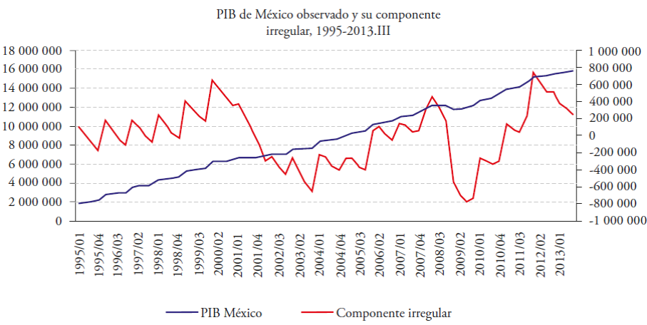
Source: Authors’ elaboration with exit data from SAS.
Figure 3 Behavior of Mexico’s GDP observed and its irregular component.

Source: Authors’ elaboration with exit data from SAS.
Figure 4 Behavior of the Exports sent to the United States and its irregular component.

Source: Authors’ elaboration with exit data from SAS.
Figure 5 Behavior of the United States GDP observed and its irregular component.
As observed in Figures 3, 4 and 5, the irregular component has been extracted and it seems that these filtered series move and return to constant average values throughout time.
The strength and sense of the existing relation between two variables was determined through the correlation coefficient: the larger the value of the coefficient is, the stronger is the relation between the variables and can take on positive or negative values, depending on the value of each observation compared to the average observed. The correlation matrix shows the following values (Table 1):
Table 1 Coefficients of correlation of the Irregular Components.
| Coeficientes de correlación de Pearson (r xy) | |||
| Variables | Comp. Irregular del PIB de México |
Comp. Irregular de las Exportaciones |
Comp. Irregular del PIB de Estados Unidos |
| PIB México | 1.00000 | 0.67295 | -0.14462 |
| Valores irregulares de suavizado | <0.0001 | 0.1814 | |
| Exportaciones | 0.67295 | 1.00000 | 0.08683 |
| Valores irregulares de suavizado | <0.0001 | 0.4239 | |
| PIB de Estados Unidos | -0.14462 | 0.08683 | 1.00000 |
| Valores irregulares de suavizado | 0.1814 | 0.4239 | |
Source: Authors’ elaboration with exit data from SAS.
The correlation between the irregular components of Mexico’s GDP and the exports sent to the United States is positive, which implies that when increasing one variable, the other also increases. The same happens for the United States exports and GDP. This is the contrary case concerning the relation of the irregular components of each country’s GDP.
In terms of the proportion of shared or explained variability determined by the coefficient of determination , the proportion of variance shared between Mexico’s GDP and the exports sent to the United States is 0.4528, while the variability between Mexican exports and the United States GDP is 0.0075.
Torres (2000) performed a study of the relation between exports and the Mexican GDP for the period of 1980-1997, and points out that the exports seem to be countercyclic, which suggests that the economic activity (GDP) is not the force that predominates over this variable. Concerning the relation between the economic cycles of Mexico and the United States, he states that this relation becomes less clear since 1987.
Almendra (2007) analyzes the cyclic fluctuations of the Mexican economy and shows that the cycle of exports is countercyclic and that it is also ahead by three trimesters with regards to the GDP cycle. Cuadra (2008) makes a description of the main stylized facts of the Mexican economic cycle and concludes, same as Almendra, that exports show a countercyclic pattern. The author also points out that for the period of 1999-2006 a high degree of synchronization was present between the economic cycles of Mexico and the United States.
We can derive from this that the coefficient of correlation found between exports and the Mexican GDP gives an idea of the existence of some positive relation between the irregular components of these variables, since they reflect that when one increases the other responds in a direct sense. On the other hand, it can be highlighted that there is no degree of incidence as such that could corroborate, at least in terms of the correlation found, that economic shocks in the United States can affect the exporting sector and, therefore, the Mexican economy.
Conclusions
The results obtained allow the following conclusions:
The first is about the relationship there is between Mexico’s GDP and the exports sent to the United States, which implies that any disturbance that happens in the exporting sector will have an influence on the Mexican GDP. The magnitude will depend, among other things, on the participation that they have in generating the GDP, as well as the composition and dragging effect towards the other productive sectors. In this case, the average participation for the study period of exports in the Mexican GDP is 5.36 %; and, second:
Given the trade relation between exports and the United States economy shown at the beginning of the study, anyone would think that the ups and downs in that country would be reflected automatically in the behavior of exports. However, the coefficient of correlation found indicates that this sector is scarcely vulnerable to any shock in that economy, which leads us to conclude that for this period the demand in the United States for Mexican exports is scarcely variable in time, and, therefore, Mexico’s economic growth through exports is not influenced by the United States economy.
REFERENCES
Almendra Arao, Genaro. 2007. Las Fluctuaciones Cíclicas de la Economía Mexicana. Colegio de Postgraduados, Campus Montecillo. México. 114 p. [ Links ]
Almendra-Arao, y A. González Estrada. 2008. Soluciones explícitas para el Filtro estadístico Hodrick-Precott. In: Revista mexicana de Economía agrícola y de los Recursos Naturales. Universidad Autónoma Chapingo. Volumen 1, Núm. 1, México. [ Links ]
Balaguer J., and Manuel Cantavella-Jordá. 2001. Examining the export-led growth hypothesis for Spain in the last century. Applied Economic Letters. Vol 8. Num 10. [ Links ]
Balaguer J. , and Manuel Cantavella-Jordá. 2004. Structural change in exports and economic growth: cointegration and causality analysis for Spain (1961-2000). Applied Economics, vol 36 num 5. [ Links ]
Cuadra, Gabriel. 2008. Hechos Estilizados del Ciclo Económico en México: En: Documentos de Investigación. Banco de México. Núm. 14, México. [ Links ]
Cuadros R. Ana M. 2000. Exportaciones y Crecimiento Económico: Un análisis de causalidad para México. Estudios Económicos, El Colegio de México A.C. vol.15, No.001, 37-64. [ Links ]
Chow, P. C. Y. 1987. Causality between export growth and industrial development: Empirical evidence from the NICs. Journal of Development Economics. vol. 26, num. 1, 55-63. [ Links ]
Donoso y Martín. 2004. Exportaciones y Crecimiento Económico: El caso de España. In: Serie Economía Internacional. Madrid España. Instituto Complutense de Estudios Internacionales, Septiembre. [ Links ]
Donoso y Martín. 2009. Exportaciones y crecimiento económico: estudios empíricos. In: Serie Economía Internacional. Madrid España. Instituto Complutense de Estudios Internacionales, Mayo. [ Links ]
Feder, G. 1982. On exports and economic growth. Journal of Development Economics. Vol. 12, Issue no. 1-2, pp: 59-73. [ Links ]
Guerrero Guzmán, Víctor Manuel. 2011. Medición de la Tendencia y el Ciclo de una serie de tiempo económica, desde una perspectiva estadística. En: Realidad, Datos y Espacio, Revista Internacional de Estadística y Geografía. INEGI. Volumen 2, Núm. 2, México. [ Links ]
Granger, C. W. J. 1969. Investigating Causal Relations by Econometric Models and Cross-spectral Methods. Econometrica. 37 (3): 424-438. [ Links ]
Hodrick R. J., and E. C. Prescott. 1997. Postwar U.S. Business Cycles: An Empirical Investigation. Journal of Money, Credit and Banking, Vol. 29, No. 1. pp: 1-16. [ Links ]
Fujii, Candaudap y Gaona. 2005. Exportaciones, Industria Maquiladora y Crecimiento Económico en México a partir de la década de los noventa. In: Investigación Económica. Núm. 254, D.F. México. Universidad Nacional Autónoma de México. [ Links ]
INEGI (Instituto Nacional de Geografía y Estadística e Informática). Banco de Información Económica. Indicadores de Coyuntura. Balanza Comercial de México. www.inegi.com.mx. Página consultada: 1 de Agosto 2014. [ Links ]
Krueger, A. 1980. Trade policy as an input to development. American Economic Review, vol. 70, No. 2. [ Links ]
Meza Carvajalino, Carlos Arturo. 2012. Econometría de Series de Tiempo: elementos y fundamentos, Editorial Académica Española, Alemania. [ Links ]
Pedregal D. J., and P. C. Young. 2001. Some comments on the use and abuse of the Hodrick Prescott filter. Review on Economic Cycles, Vol. 2, No. 1. [ Links ]
Ramírez, Javier. 2005. La economía mexicana y el sector externo: Tendencias y Cointegración. In: Estudios Económicos de Desarrollo Internacional. Volumen 5, Núm. 22, México. [ Links ]
Rodríguez y Venegas. 2011. Efecto de las exportaciones en el crecimiento económico de México: Un análisis de cointegración, 1929-2009. En EconoQuantum. Volumen 7, Núm. 2, Zapopan. Universidad de Guadalajara. [ Links ]
SE (Secretaria de Economía). Subsecretaria de Comercio Exterior. https://www.gob.mx/cms/uploads/attachment/file/336605/Anual-Exporta-dic2014.pdf. página consultada: 1 de Septiembre del 2014. [ Links ]
Torres García, Alberto. 2000. Estabilidad en variables nominales y el ciclo económico: El caso de México. In: Documentos de Investigación, Banco de México. Núm. 3. [ Links ]
Tyler W. G. 1981. Growth and export expansion in developing countries: Some empirical evidence. Journal of Development Economics, 1981, vol. 9, num. 1, 121-130. [ Links ]
2It is said that a variable Y2 causes Y1 in the Granger sense, if the predictor of Y1 built from its own past values can be improved when the past values of Y2 are included in its prediction (Granger, 1969).
Received: March 01, 2014; Accepted: August 01, 2017
 Este es un artículo publicado en acceso abierto bajo una licencia Creative Commons
