


 nova página do texto(beta)
 Inglês (pdf)
 Artigo em XML
 Referências do artigo
 Enviar este artigo por email
 Citado por SciELO
  Similares em
SciELO
Similares em
SciELO 
 Permalink
PACS: 83.10.Mj; 83.85.Cg; 83.85.Jn
1. Introduction
The viscosity of a fluid describes the internal drag forces within the fluid as it is subjected to stress 1. Accurate descriptions of viscosity have a broad range of applications, from the characterization of blood flow, as it relates to corollary heart disease, to optimizing lubricants for mechanical systems 2,3. Isaac Newton first described fluid viscosity in his 1687 Principia, where he stated Newton’s Law of Viscosity, describing the response of a continuous, incompressible fluid to shear stress 4. In the 1840s, the Navier-Stokes equation was derived and used to describe the diffusion of totally conserved quantities through a continuous fluid 5. In 1866, James Maxwell reported experimental results which verified his earlier calculations showing viscosity of a gas is dependent on the mean free path of its particles 6. Later, a microscopic description of diffusion grounded in Robert Brown’s 1827 observations of pollen particles randomly moving was independently developed by Albert Einstein in 1905 and by Marian Smoluchowski in 1906, resulting in the Einstein-Smoluchowski relation describing the probe diffusion coefficient 7,8. Through George Stokes’ 1851 derivation of Stokes’ Law, the diffusion coefficient is related back to the fluid viscosity describing the frictional drag felt by individual particles in a continuous media 9.
In the broadest mathematical formalism, viscosity is given by the viscosity tensor, μ, in
relating the viscous stress tensor for a fluid, τ, and strain rate tensor, ϵ10. For Newtonian fluids, μ has three independent components: the bulk, dynamic, and rotational viscosities which describe fluid response to compressive forces, resistance to shear, and the coupling between flow and individual particle rotations, respectively 10. As was done historically, compatible expressions for dynamic viscosity and related quantities can be derived under two different theoretical models of fluids. The first model is a macroscopic, continuum one relating diffusion to concentration gradients. The second is a statistical, Brownian motion model of single particle diffusion at local scales. Introduction of the term viscosity from both perspectives is followed by three different approaches to experimentally determine the viscosity of a Newtonian fluid. These three experimental methods range in scales from nm to cm and from ns to seconds. The shear stress of solutions of glucose at different concentrations was studied using a rheometer. For the probing of local viscosity, translational and rotational diffusion of Rhodamine-110 were observed in glucose solution utilizing Fluorescence Correlation Spectroscopy (FCS) and time-resolved anisotropy measurements, respectively.
1.1. Continuous fluid
Empirically verified by Newton, Newton’s Law of Viscosity is
where F is the force in contact with a liquid over a cross sectional area A,
The dynamics of fluids, including diffusive processes which depend on the viscosity of the fluid, can also be described using the Navier-Stokes equation. Let us begin from the Cauchy Momentum Equation, a statement of conservation of momentum for a continuum:
where p = ρ u is the momentum density defined by the mass density (ρ) times velocity (u), t is time, J p is the momentum density flux out of the volume, and s is a source term corresponding to stresses and forces imparting momentum on the system. Rewriting in terms of ρ, u, the material derivative D/Dt, the sum of externally-caused accelerations, g, the pressure, p, and the stress tensor, τ, we obtain
Plugging in Eq. (1), where
Taking the limit of an incompressible, Newtonian fluid, ρ is a constant and
Finally, we take the limits in which the external and hydrostatic force contributions are negligible and there is no net fluid flow. The net result is that the material derivative reduces to the partial time derivative and the external force terms become 0, leaving
This is the linear Navier-Stokes momentum density equation for an incompressible, non-convecting fluid subjected to viscous forces 14. Equation (7) is essentially the momentum diffusion equation and is closely related to Eq. (2). A similar analysis can be performed beginning from the conservation of amount of fluid in terms of concentration, C, with no sources:
Making use of the empirically verified Fick’s First Law,
where D is defined as the translational diffusion coefficient, we obtain
This is the non-convective, un-sourced diffusion equation in terms of concentration, or Fick’s Second Law for constant D1,15. D describes the rate at which a substance (either a continuum or a single particle) diffuses through medium. D depends on the viscous drag force exerted by the fluid. D can be explicitly related to the viscosity experienced by a probe through the Stokes-Einstein relation discussed in the next section 16.
1.2. Thermally-driven random walk
Viscosity can also be defined by considering individual particles undergoing Brownian motion in media. In Brownian motion, each individual probe particle undergoes an effective random walk driven by thermal energy 17. This model allows a derivation of the diffusion equation from a microscopic, statistical perspective which matches the continuum case. Let us consider a particle randomly walking in space with probabilities p and q to travel either right or left in the
By doing a Taylor expansion to first order in t and second order in x in the continuous limit (small τ and δ), we obtain that the first non-vanishing contribution leads to
the convective diffusion equation, with translational diffusion coefficient D = δ 2/2τ18. In our case of unbiased walking, p = q and this reduces to
Finally, assuming that D is the same in each direction and summing over the three Cartesian coordinates, we obtain
the analog of Eq. (10) for a single probe diffusing through a fluid. These equations describe the same phenomena under the substitution P = C, or taking particle concentration for many particles as a probability distribution. This is seen in their shared solution
where
is found, where
Through the considerations of random forces acting on particles undergoing Brownian motion, Einstein and Smoluchowski independently arrived at the fluctuation-dissipation relation
where
and by
where R is the probe particle’s radius 13,16.20. Combination of Eq. (18) or (19) with Eq. (17) directly relates D or
1.3. Scaling Law
At lengthscales associated with individual random walkers, scaling laws for diffusion become suitable. Such is the case in crowded and disordered intracellular environments, where additional effective drag interactions between the probe and the individual solution molecules become important. Thus, the definition of an effective local viscosity, described by the diffusion coefficient and which accounts for these interactions, becomes relevant 21. To introduce this effect and the introduction of active transport effects or Levy flights at the probe level and bridge the gap between the macroscopic and local viscosity scales, it is useful to consider the space-fractional version of the diffusion equation, Eq. (13), given by
Here,
Consider f0, the drag experienced by a probe diffusing in an infinitely dilute polymer solution. As polymers are more rigid than the solvent, their presence in solution provides an additional drag term depending on their diffusion characteristics. Additionally, this increase is magnified at higher concentrations since the presence of polymers will effectively increase the drag experienced by other polymers as well. If we now consider two increments in polymer concentration, dC, then we can make the assumption that each increment increases f by an amount a(C)fdC, where a(C) is a concentration-dependent modifier to f. After the first increment, f = f0 is then modified such that
Then after the second increment,
or
Rearranging
Finally, taking the limit
Substituting this into Eq. (17) yields
Where D0 is the probe diffusion coefficient corresponding to f0 at infinite polymer dilution. Assuming the hydrodynamic interactions between polymers to scale similarly to those for hard spheres described by Mazur and van Saarloos, the integral in Eq. (26) can be shown to scale with βC1-2x23. Here, β is an average of higher-order interactions determining how readily a solution’s viscosity changes with polymer solution and x is a scaling factor depending directly on the effective radii of gyration of both the polymers and the probe 23,24. Substituting 1 - 2x = v, we finally obtain
the empirically verified universal scaling law for diffusion in polymer solutions 24,25,26. Such a scale-flexible relationship has been suggested through experiments under several polymer models, namely reptation-scaling treatment, hydrodynamic screening, and hydrodynamic scaling 27,28,29. Combining with Eqs. (17), (18), and (19), we obtain the normalized local viscosity as a function of osmolyte concentration, given by
with η0 as the viscosity at infinite dilution of the solute polymer. We use this key equation to determine the concentration dependence of viscosity, which is compared through various experimental methods that probe viscosity at various length- and time- scales.
2. Probing Viscosity Experimentally
To experimentally verify the theoretical agreement between the macroscopic and the local viscosity, and to test the validity of Eq. (27), we independently probe different timescales and lengthscales associated with each treatment. The macroscopic view of viscosity was assessed using rheometer measurements at a lengthscale of a few centimeters and a timescale close to seconds. Single particle tracking methods should be ideal to study viscosity from the microscopic perspective of Brownian motion; however, technical difficulties restrict most implementations of these methods for random walks in two dimensions 30. Therefore, alternative methods have been developed which simplify the determination of the diffusion coefficient. One of these methods is Fluorescence Correlation Spectroscopy (FCS), which probes the diffusion at sub-millisecond timescales and which can be implemented using inexpensive Field Programmable Gate Array (FPGA) boards as FCS hardware correlators 31,32. FCS is accomplished by correlating the time dependent fluorescence intensity as fluorescent markers diffuse through a small detection volume. Another method, time-resolved fluorescence anisotropy, allows for the study of rotational diffusion through the measurement of random re-orientations of the tracer particle. By considering the angular rotation of the particle, a similar viscous effect is observed. Thus, time-resolved anisotropy measures the tracer’s rotational diffusion coefficient, allowing determination of viscosity at the nm lengthscale and ns timescale 33. Following is a brief introduction to these methods and brief descriptions of the materials used.
2.1. Glucose solutions and rhodamine-110 probe
To probe the viscosity at different timescales and lengthscales, we created various solutions of D-Glucose (Table I) ranging from

For steady state fluorescence spectroscopy, Rhodamine-110 (Table I) was brought into solution and used at 2 nM or 100 nM solutions for FCS and time resolved measurements. Rhodamine-110 is a particularly bright fluorophore with a well-characterized fluorescence lifetime, making it an excellent candidate for these experiments 34.
For probe-based methods, the reporter molecules’ fluorescent properties must not change under the conditions of the experiments. Thus, the steady-state fluorescence excitation and emission spectra at all concentrations of glucose were characterized. The excitation and emission wavelengths for both the 5% and 30% D-Glucose solutions, seen in Fig. 1A, were found to be 487 nm and 521 nm, respectively.
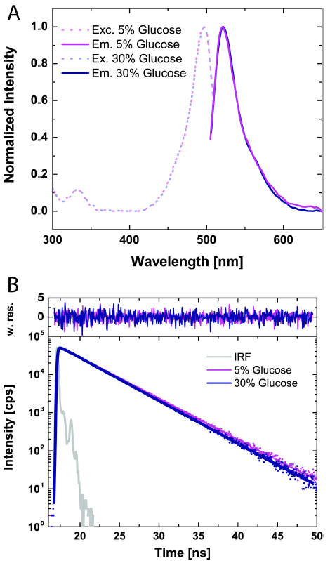
Figure 1. (A) Fluorescence excitation and emission spectra of Rhodamine-110 in 5% and 30% (w/v) D-Glucose solutions. In both cases, the peak excitation wavelength was 487 nm with peak emission wavelength at 521 nm. (B) Corresponding time-resolved fluorescence decays and fit function Eq. (40). Lifetimes for the 5% and 30% D-Glucose solutions exhibited the same behavior with lifetimes of 3.964 and 3.978 ns, respectively. Instrument response function (IRF) is shown in gray.
No major difference is observed in the normalized spectra, assuring that the fluorescence properties of Rhodamine-110 are independent of the environment.
Spectral measurements are mostly insensitive to dynamic quenching, particularly if the concentrations of the solutions of Rhodamine-110 are not carefully controlled. Thus, to show that quenching does not occur or is minimally present in D-Glucose solutions, we measured the time-resolved fluorescence decays of Rhodamine-110 at all D-Glucose solution concentrations. Figure 1B shows representative normalized fluorescence decay spectra at 5% and 30% D-Glucose solutions, with the corresponding weighted residuals on top after the model function Eq. (40) is used for fitting.
The 5% and 30% solutions show very similar decays with no major changes in the fluorescence lifetimes derived from Eq. (40). Dynamic quenching would cause a shift towards shorter lifetimes as the concentration of the quencher increased. This effect follows the Stern-Volmer relation 35. From this, it was concluded that Rhodamine-110 suffered minimal collision-induced deactivation processes.
2.2. Rheometer
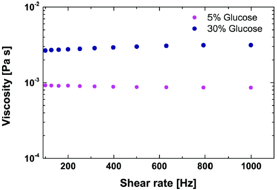
Classical rheometry experiments consist of using a small amount of solution as a lubricant between two rotating plates. By measuring the resistance to flow imparted on the plates by the solution, the dynamic viscosity can be determined through Eq. (2). Small amounts of D-Glucose solutions were placed between the two plates of a T.A. Instruments (Rheolyst model) AR1000-N Rheometer and measured using multiple shear rates in order to determine the viscosity. The typical response of a Newtonian fluid whose shear rate and shear stress follow a linear relationship is seen when we plot the viscosity in Fig. 2 as a function of the shear rate. This observed response gives a constant viscosity, indicating a lack of viscoelastic effects under varying levels of stress. As expected, the viscosity increased with the increase of D-Glucose concentration, and even at 30% D-Glucose the solution still behaved as a Newtonian fluid.
2.3. Fluorescence correlation spectroscopy
Fluorescence correlation spectroscopy utilizes dilute solutions in the picomolar to micromolar range of diffusing particles to measure and correlate deviations from steady-state average fluorescence intensity in a small confocal volume. The diffusing particles either are fluorophores or are labeled with fluorophores, which are excited by lasers and subsequently re-emit light, giving rise to the intensity fluctuations. The correlation allows the determination of average particle numbers, photochemical effect timescales, diffusion times, and other parameters at the nanoscale. Choosing concentrations for measurement relies on a balancing of the factors that fluctuations from individual particles scale in the Poissonian distribution as
The theory of FCS can be summarized as follows. Consider a total-time (T) averaged fluorescence signal
Then, deviations from the average fluorescence are given by
This can be re-written as and integral over the effective detection volume
where r is the position vector, W(r) is a function describing the geometry of the detection or confocal volume, and δ(s) characterizes individual fluctuation contributions due to parameters s which can include fluctuations in quantum yield, absorption cross-sections, and, in our case, local concentration 36. Plugging this into the autocorrelation function which describes the self-similarity of a signal after a time τ, defined by
yields
This equation can then be solved by quantifying the parameters s for a given experimental setup, leading to the separability in δ(s) of contributing factors with sufficiently differing timescales and simplifying the problem 36.
For these experiments we use a home built microscope adapted for confocal FCS measurements consists of a single diode laser (Model LDH-D-C- 485 at 485 nm; PicoQuant, Germany) operating at 40 MHz on an Olympus IX73 body. Freely diffusing Rhodamine-110 molecules are excited as they pass through the focal point of a 60X, 1.2 NA collar-corrected (0.17) Olympus objective. The power at the objective was set at 120 μW. The emitted fluorescence signal was collected through the same objective and spatially filtered using a 70 μm pinhole to define an effective confocal detection volume. The emitted fluorescence was divided into parallel and perpendicular polarization components through band pass filters, ET525/50 for detecting “green” fluorescence photons. Two green PMA Hybrid detectors (PMA 40 PicoQuant, Germany) were used for photon counting. A time-correlated single photon counting (TCSPC) module (HydraHarp 400, PicoQuant, Germany) with a Time-Tagged Time-Resolved (TTTR) mode and two synchronized input channels were used for data registration and off-line fluorescence fluctuation analysis, similar to what has been used before 37. Software correlation of TTTR data files was carried out to compute correlation curves that could cover over 12 orders of magnitude in time with a multi-tau algorithm 38.
It can be shown that the analytic solution to describe fluorescence correlation in our confocal setup is given as
where N is the mean number of molecules in the detection volume,
xT is the fraction of molecules
exerting triplet state kinetics with characteristic time
tT ,
tc is the correlation time,
where the detection volume is defined by the 1/e2 radii denoted
in terms of
Both fluorescence triplet state kinetics and translational diffusion, resulting in local concentration fluctuations, were considered, allowing separability of δ(s) and leading to
where Gtriplet is the term in parentheses in Eq. (34) multiplying the term corresponding to Gdiffusion. Thus, Eq. (34) represents the correlation function of a single tracer species diffusing in a chemically equilibrated solution detected in a confocal volume described by a three-dimensional Gaussian function.
Finally, the diffusion coefficient can be determined using the diffusion time tdiff as
D is again related to the viscosity through Eq. and (18).
We use FCS, with Rhodamine-110 as our tracer particle, to determine the diffusion coefficient
as molecules travel across a confocal volume with a
1/e2 radius of ~ 250 nm in sub millisecond
timescales. As molecules traverse the confocal illumination volume, they emit
light after being excited by a pulsed laser. When they exit the confocal volume
the signal for that molecule stops. This causes fluctuations in intensity, which
are recorded by the photon detectors. When the fluorescence intensity is
correlated, these fluctuations generate a decay function that can be modeled
with Eq. (34), from which the diffusion coefficient can be extracted. From this
diffusion coefficient, the viscosity of the solution as sensed by the probe is
found. Fig. 3 shows the correlation
function and the model fits for Rhodamine-110 in
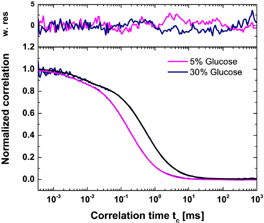
Figure 3. Overlay of Fluorescence Correlation Spectroscopy curves and the corresponding fit model function Eq. (34) for Rhodmaine-110 in 5% and 30% (w/v) D-Glucose solutions. The confocal volume’s ratio of its height to its waist is given as a constant 4.609 for both concentrations. The time of diffusion for Rhodamine-110 was 0.192 ms for the 5% solution and 0.597 ms for the 30% solution. The fraction of triplet states, given by xT, was 0.093 for 5% and 0.130 for 30%. The relaxation time tT for 5% and 30% are 0.003 to 0.008 ms, respectively.
2.4. Time-resolved anisotropy
The rotational diffusion is affected by the rotational drag force exerted on the probe by D-Glucose. This effect can be monitored by studying the rotational correlation time in time-resolved fluorescence anisotropy measurements. A brief theoretical treatment of this technique is as follows: consider a population of fluorophores, ni , of species i. Then ni,+ + ni,0 = ni , where ni,+ is the number of particles in the excited state and ni,0 is the number in the ground state.
Given the fluorescence lifetime, τi , and the excitation intensity, I(t), the rate of change in the excited state population is given by the well-known rate equation,
Solving this equation for decay after an excitation pulse (such that I(t > 0) = 0 and we need only consider t > 0) yields
Utilizing the facts that the fluorescence intensity is directly proportional to the number of excited states of fluorophores and that the total intensity is the sum of species contributions, the fluorescence intensity decay can be generally treated as a multi-exponential decay function using
Here xi are the pre-exponential intensity factors.
For time-resolved anisotropy, the parallel and perpendicular decay components of the fluorescence,
where F(t) is the time-resolved fluorescence decay at magic angle conditions following Eq. (40) and r(t) is the time-dependent anisotropy. In terms of the measured parallel and perpendicular components of the fluorescence decay, r(t) is given by
where G is an instrumental correction factor to account for changes in the
the detection efficiency given wavelength and polarization. Here,
FVV and
FVH are
where r0 =
Ʃibi
is the fundamental anisotropy and
bi are the fractional
anisotropies that decay with correlation times
ρi , which in turn are
related to the rotational diffusion coefficient
thus, relating the rotational correlation time directly to the dynamic viscosity as the particle rotates. More complex expressions are predicted for nonsymmetric probe particles, but this goes beyond the scope of the exercise. In our case, we assume that the tracer particle, Rhodamine-110, is a sphere.
To assure that photophysical factors do not affect our probe experiments, we first measured the steady state fluorescence spectra, followed by ensemble time-correlated single-photon-counting (eTCSPC) using a Fluorolog3 spectrofluorometer in T-shape with a PDX detector (Horiba Yvon, USA) system. The light from a xenon lamp was used to collect excitation and emission spectra using an excitation monochromator set at 494 nm and an emission monochromator at 520 nm, accordingly. The scanning monochromator slit was set to 1 nm while the fixed monochromator slit was set to 5 nm. Spectra measurements were collected under magic angle conditions by using a vertical polarized excitation source and placing an emission polarizer to 54.7°. For time-resolved fluorescence and time-resolved anisotropy measurements, the excitation source was a NanoLED 485 nm diode laser (NanoLED 485L, Horiba, Country) operating at 1 MHz. The emission monochromator slit was set to 16 nm (emission path). The signal of the photon counting unit was sent to a FluoroHub-B with a bin width of 55 ps. Fluorescence intensity decays in all polarizations were collected to determine the proper detection efficiency factor and determine time-resolved anisotropy. Figure 4 shows the time-resolved anisotropy decays of Rhodamine-110 in 5% and 30% D-Glucose solutions. As expected, the rotational diffusion shows a slowing behavior in the anisotropy decay as the concentration of D-Glucose increases. By analyzing the decay function and fitting it with the model function, Eq. (44), the average rotational correlation time is found. Then, Eq. (45) is used to calculate the viscosity.
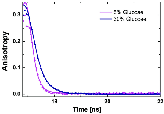
Figure 4. Overlay of time-dependent anisotropy decays and the corresponding fit model function Eq. (44) for Rhodmaine-110 in 5% and 30% (w/v) D-Glucose solutions. From this specific correlation, the rotational speeds in the 5% and 30% D-Glucose solutions were 100 ±0.002 ps and 385 ±0.001 ps, respectively.
2.5. Error analysis
Experimental reproducibility was evaluated using triplicated solutions of Rhodamine-110 in the FCS experiments. Each measurement was carried out at different times and with different starting stock conditions. The mean and standard deviation amongst these results was used to report our parameters. The uncertainty of experimental error was manifested using the standard deviation.
The statistical uncertainties of the fits from the time-resolved anisotropy decays were estimated by exploring the
where N is the number of fit points and
To evaluate the conditions of the experiments and how that introduces potential errors, we used the data collected with the Rheometer at different shear frequencies. Frequencies ranging from 0-1000 Hz were used to evaluate the mean determined viscosity and standard deviation as representations of uncertainty in the methodology.
3. Discussion
Different methodologies capture the drag frictional force at various time and length scales. For example, Fig. 5A shows a linear correlation between the rotational and translational diffusion time. These measurements show a link between the interactions that occur at the nanoscale range to the interactions that occur over the span of hundreds of nanometers in the confocal illumination volume. This relationship between rotational and translational diffusion can further be seen through the fact that both measurements sense the same shear viscosity. Both methods do not exert significant stress on the fluid, thus it can be considered the ideal shear-less condition of a Newtonian fluid. While the rheomtery does induce shear stress, we noted that there is no dependence of the viscosity on this stress.
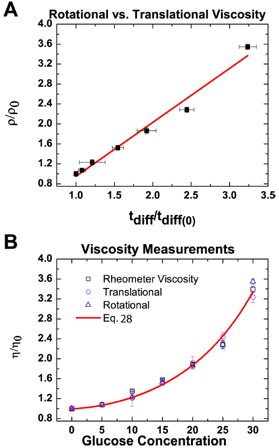
Figure 5. Viscosity comparisons. A) A direct comparison of the measurement rotational motion with that of the translational motion of Rhodamine-110. B) A representation of the normalized viscosity change as a function of D-Glucose concentration for all three experiments. The red curve represents the fit for averaged data, given by Eq. (28).
3.1. Power law of viscosity
To reduce errors in calibration, the viscosity at different concentrations of Glucose was normalized to the viscosity of the buffer solution (η/η0) (Fig. 5B). Comparing the viscosity as derived from different experimental measurement, we observed that all values follow an exponential growth curve as a function of the concentration of D-Glucose. The exponential growth in Fig. 5B was fit with Eq. to evaluate the expected scaling law dependence of viscosity. Fitting the three data sets independently yields the results given in Table II. Due to the apparent similarity in the data as shown in Fig. 5A, the average of the fit parameters was calculated and the averaged data was also fit all together, yielding similar values also found in Table II. Note that v is specific to the dimensions and type of solute osmolyte and probe used, given the assumptions of Eq. such as the dependence on the radii of gyration in x. However, we determined that this parameter is actually independent of dimensionality because the probe and probeless methodologies were able to show similar values for viscosity. The beta value is a measure of how readily the solution changes in viscosity based on its concentration.

3.2. Closing Remarks
In summary, for a non-compressible Newtonian fluid, in which viscosity is independent of stress, probe viscosity (local microscopic) and shear viscosity (macroscopic) are identical. While probing the local viscosity, the probe does not exert stress while moving through the media; thus, no turbulent or convective effects must be accounted for, consistent with fluid behavior for low Reynolds number hydrodynamics. Combining classical rheology, FCS, and time-resolved anisotropy allows us to show that probe diffusion senses an effective local viscosity consistent with the macroscopic definition of shear viscosity. A similar approach can be applied to complex fluids, where the scaling behavior is relevant, and thus characterize the possible divergence between the local and macroscopic viscosities. Furthermore, these methodologies should be viable for future measurements of viscosities in compressible or other non-Newtonian fluids with either no or only small modifications to the experimental setup, assuming those materials are otherwise suitable for fluorescence techniques. For example, an external pressure source could be introduced to compress a sample in a T-shaped confocal setup for FCS and anisotropy measurements without interfering with the paths of the lasers to the sample or of light from the sample to the detectors. To this end, the modularity of such setups is a great aid. Additionally, classical rheometry experiments for comparison are also usable in pressure-sensitive experiments and, in fact, Maxwell’s study of gas viscosities utilized such a setup with glass disks 6.

