1. Introduction

The simple plane pendulum constitutes an important physical system whose analytical solutions are well known. Historically the first systematic study of the pendulum is attributed to Galileo Galilei, around 1602. Thirty years later he discovered that the period of small oscillations is approximately independent of the amplitude of the swing, property termed as isochronism, and in 1673 Huygens published the mathematical formula for this period. However, as soon as 1636, Marin Mersenne and René Descartes had stablished that the period in fact does depend of the amplitude ¹. The mathematical theory to evaluate this period took longer to be established.

The Newton second law for the pendulum leads to a nonlinear differential equation of second order whose solutions are given in terms of either Jacobi elliptic functions or Weierstrass elliptic functions^{1,2,3,4,5,6,7}. There are several textbooks on classical mechanics ^8,9,10, and recent papers ^11,12,13, that give account of these solutions. From the mathematical point of view the subject of interest is the one of elliptic curves such as y ² = (1-x²)(1-k² x²), with k2≠0,1, the corresponding elliptic integrals∫0xdx/y and the elliptic functions which derive from the inversion of them. Generically the domain of the elliptic functions is the complex plane C and they depend also on the value of the modulus k. The theory began to be studied in the mid eighteenth century and involved great mathematicians such as Fagnano, Euler, Gauss and Lagrange. The cornerstone in its development is due to Abel ¹⁴ and Jacobi ^15,16, who replaced the elliptic integrals by the elliptic functions as the object of study. Since then they both are recognized jointly as the mathematicians that developed the elliptic functions theory in their current form and to the theory itself as one of the jewels of nineteen-century mathematics.

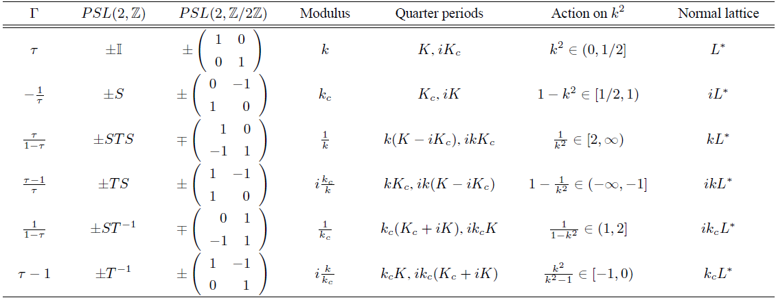
Because the solutions to the simple pendulum problem are given in terms of elliptic functions and the founder fathers of the subject taught us all the interesting properties of these functions, it can be concluded that all the characteristics of the different type of motions of the pendulum are known. This is strictly true, however most of the references on elliptic functions (see for instance ^2,3,4,5,6,7 and references therein) focus, as it should be, on its mathematical properties, applying just some of them to the simple pendulum as an example. In this paper we review part of the analysis made by Klein ¹⁷, who studied the properties that the transformations of the modular group Γ and its congruence subgroups of finite index Γ(N) have on the modular parameter τ, being the latter a function of the quarter periods K and K_c which in turn are determined by the value of the square modulus k². Our main interest in this paper is to accentuate the physical meaning that these transformations have in the specific case of the simple pendulum, in our opinion this is a piece of analysis missing in the literature.

For our purposes the relevant mathematical result is that the congruence subgroup of level 2, denoted as Γ(2), is of order six in Γ and therefore a fundamental cell for Γ(2) can be formed from six copies of any fundamental region F of Γ produced by the action of the six elements on the set of modular parameters τ that belong to F. Each of these copies is distinguished from each other, according to the functional form of the modulus k² the six transformations leave invariant, being they: k², 1- k², 1/ k², 1-1/ k², 1/(1- k²) and k²/(k² -1). Interestingly these kind of relations appear in other areas of physics under the concept of duality transformations, nomenclature we will use here. This result can be understood from different mathematical points of view and provides a link between concepts such as lattices, complex structures on the topological torus T2, the modular group Γ and elliptic functions. In the appendices we review briefly the basics of these concepts in order to keep the paper self contained as possible, emphasizing in every moment its role in the solutions of the simple pendulum. From the physical point of view, the pendulum can follow basically two kind of motions (with the addition of some limit situations), the specific type of motion depends entirely on the value of the total mechanical energy kE2, if 0<kE2<1 the motion is oscillatory and if 1<kE2<∞ the motion is circulatory. Therefore in the problem of the simple pendulum, there are two relevant parameters, the square modulus k² of the elliptic functions that parameterize its solutions in terms of the time variable, and the total mechanical energy of the motion kE2. As we will discuss throughout the paper, the relation between these two parameters is not one-to-one due to the duality relations between the different invariant functional forms of k². For instance, for an oscillatory motion whose energy is 0<kE2<1, it is possible to express the solution in terms of an elliptic Jacobi function whose square modulus is k², 1 - k², 1/k², etc., in other words, the duality symmetries between the functional forms of the square modulus k² induce different equivalent ways to write the solution for a specific physical motion of the pendulum. The nature of the time variable also plays an important role in the equivalence of solutions, it turns out that whereas some solutions are functions of a real time, others are functions of a pure imaginary time. In this paper we will discuss all these issues and we will write down explicitly several equivalent solutions to describe a specific pendulum motion. These results constitute an example in classical mechanics of a broader concept in physics termed under the name dualities. It is worth mentioning that some of the results we present here are already scattered throughout the mathematical literature but our exposition collects them together and is driven by a golden rule in physics that demands to explore all the physical consequences from symmetries. Notwithstanding some formulas have been worked out specifically for building up the arguments given in here and to the best knowledge of the author they are not present in the available literature. As an example, we obtain a single solution that describes the motions of the simple pendulum as function of a pure imaginary time parameter, and we show it can be obtained through an S-duality transformation from a single formula that describes the motions of the simple pendulum for all permissible values of the total energy and which is function of a real time variable.

In a general context the duality symmetries we refer to, involve the special linear group SL(2,Z) and appear often in physics either as a symmetry of a theory or as a relationship among two different theories. Typically these discrete symmetries relate strong coupled degrees of freedom to weakly coupled ones and vice versa, and the relationship is useful when one of the two systems so related can be analyzed, permitting conclusions to be drawn for its dual by acting with the duality transformations. There is a plethora of examples in physics that obey duality symmetries, which have led to important developments in field theory, gravity, statistical mechanics, string theory etc. (for an explicit account of examples see for instance ¹⁸ and references therein). As a manner of illustration let us mention just two examples of theories that own duality symmetries: i) in string theory appear three types of dualities, and the one that have the properties described above goes by the name S-duality, being the S group element, one of the two generators of the group SL(2,Z) ¹⁹. In this case the modular parameter τ is given by the coupling constant and therefore the S-duality relates the strong coupling regime of a given string theory to the weak coupling one of either the same string theory or another string theory. It is conjectured for instance that the type I superstring is S-dual to the SO(32) heterotic superstring, and that the type IIB superstring is S -dual to itself. ii) In 2D systems there is a broad class of dual relationships for which the electromagnetic response is governed by particles and vortices whose properties are similar. In particular for systems having fermions as the particles (or those related to fermions by the duality) the vortex-particle duality implies the duality group is the level-two subgroup Γ₀(2) of PSL(2,Z) ²⁰. The so often appearance of these duality symmetries in physics is our main motivation to heighten the fact that in classical mechanics there are systems like the simple pendulum whose motions can be described in different equivalent forms related by duality symmetries.

The structure of the paper is as follows. In Sec. 2 we summarize the real time solutions of the simple pendulum system in terms of elliptical Jacobi functions. The relations between solutions with real time and pure imaginary time in terms of the S group element of the modular group Γ are exemplified in Sec. 3 and the whole web of dualities is discussed in Sec. 4. We make some final remarks in 5. There are two appendices, Appendix A is dedicated to define the modular group, its congruence subgroups and its relation to double lattices whereas in Appendix B we give some properties of the elliptic Jacobi functions that are relevant for the analysis of the solutions of the simple pendulum.

2. Real time solutions

The Lagrangian for a pendulum of point mass m and length l, in a constant downwards gravitational field, of magnitude -g g>0, is given by

where θ is the polar angle measured counterclockwise respect to the vertical line and θ˙ stands for the time derivative of this angular position. Here the zero of the potential energy is set at the lowest vertical position of the pendulum, for which θ=2nπ, with n∈Z. The equation of motion for this system is

This equation can be integrated once giving origin to a first order differential equation, whose physical meaning is the conservation of energy

Physical solutions exist only if E≥0. We can rewrite this equation of conservation, in dimensionless form, in terms of the dimensionless energy parameter: kE2≡(E/2mgl), and the dimensionless real time variable: x≡(g/l)t∈R, obtaining

Analyzing the potential, it is concluded that the pendulum has four different types of solutions depending of the value of the constant kE2. The analytical solutions in two of the four cases are given in terms of Jacobi elliptic functions and can be found for instance in ^{5,7,8,9,10,11,12,13}. The other two cases can be considered just as limit situations of the previous two. The Jacobi elliptic functions are doubly periodic functions in the complex z-plane (see Appendix B for a short summary of the basic properties of these functions), for example, the function sn(z, k) of square modulus 0 < k² < 1, has the real primitive period 4K and the pure imaginary primitive period 2iK_c , where the so called quarter periods K and K_c are defined by the Eqs. (B.2) and (B.5) respectively. The properties of the different solutions are as follows:

where the square modulus k² of the elliptic functions is given directly by the energy parameter: k2≡kE2. Here x₀ is a second constant of integration and appears when Eq. (4) is integrated out. It means physically that we can choose the zero of time arbitrarily. Derivatives of the basic Jacobi elliptic functions are given in (B.11).

Without loss of generality, in our discussion we consider that the lowest vertical point of the oscillation corresponds to the angular value θ=0, and therefore that θ takes values in the closed interval [-θm,θm], where 0<θm<π is the angle for which θ˙m=0. This means that: sinθ2∈[-sinθm2,sinθm2], where according to Eq. (4), sin2(θm/2)=kE2<1. Now according to (5) the solution is obtained by mapping ²⁷: sin(θ/2)→kE sn(x-x0,kE), where x-x0∈[-K,K], or equivalently: snx-x0,kE∈[-1,1]. With this map we describe half of a period of oscillation. To describe the another half, without loss of generality, we can extend the mapping in such a way that for a complete period of oscillation, x-x0∈[-K,3K]. Because the Jacobi function cn x-x0,kE∈[-1,1], the dimensionless angular velocity ω(x) is restricted to values in the interval [-2kE,2kE].

As an example we can choose x₀ = K, so at the time x = 0, the pendulum is at minimum angular position θ(0)=-θm, with angular velocity ω(0) = 0. The pendulum starts moving from left to right, so at x = K it reaches the lowest vertical position θ(K)=0 at highest velocity ω(K) = 2k_E and at x = 2K it is at maximum angular position θ(2K)=θm with velocity ω(2K) = 0. At this very moment the pendulum starts moving from right to left, so at x = 3K it is again at θ(3K)=0 but now with lowest angular velocity ω(3K) = -2k_E and it completes an oscillation at x = 4K when the pendulum reaches again the point θ(4K)=-θm with zero velocity (see Fig. 1). We can repeat this process every time the pendulum swings in the interval [-θm,θm], in such a way that the argument of the elliptic function sn(x, k_E ), becomes defined in the whole real line R. It is clear that the period of the movement is 4K, or restoring the dimension of time, 4Kg/l.

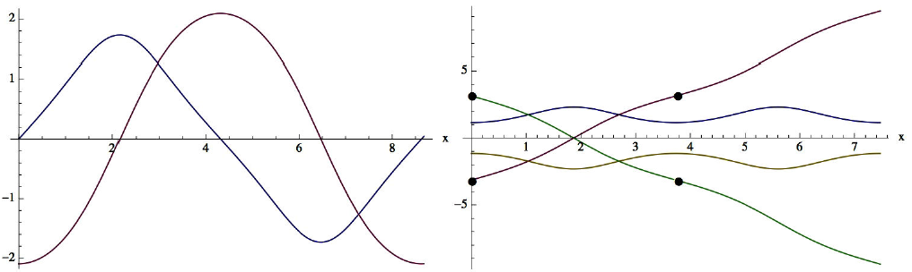
Figure 1. The first set of graphs represents an oscillatory motion of energy kE2=3∕4 with x0=K≈2.1565. θx is given by the magenta graph and it oscillates in the interval θx∈-2π/3,2π∕3. The angular velocity ω(x) is showed in blue and takes values in the interval ωx∈-3, 3. Both graphs have period 4K. The second set of graphs represents a couple of circulating motions both of energy kE2=4∕3 with x0=K/kE≈1.8676. For the motion in the counterclockwise direction, the monotonic increasing function θx is plotted in magenta, for the time interval x∈0, 2x0 it takes values in the interval θx∈[-π, π, whereas for the interval x∈2x0, 4x0 it takes values in the interval θx∈[π, 3π. The angular velocity is showed in blue, it has period 2K/k_E , is always positive and takes values in the interval ωx∈2∕3, 4∕3. The other two plots represent a similar motion in the clockwise direction. 

Of course the value of x₀ can be set arbitrarily and it is also possible to parameterize the solution in such a way that at zero time x = 0, the motion starts in the angle θm instead of -θm. In this case the mapping of a complete period of oscillation can be defined for instance in the interval x-x0∈[K,5K] and the initial condition can be taken as x₀ = -K. In the discussion of the following section we will set x₀ = 0, so at time x = 0, the pendulum is at the lowest vertical position (θ(0)=0) moving from left to right.

● Asymptotical motion (kE2=1 and θ˙≠0): In this case the angle θ takes values in the open interval (-π, π) and therefore, sin(θ/2)∈(-1,1). The particle just reach the highest point of the circle. The analytical solutions are given by

The sign ± corresponds to the movement from (∓π→±π). Notice that tanh(x-x ₀), takes values in the open interval (-1,1) if: x-x0∈(-∞,∞). For instance if θ→π, x - x₀→ ꝏ and tanh(x - x₀) goes asymptotically to 1. It is clear that this movement is not periodic. In the literature it is common to take x₀ = 0.

● Circulating motions (kE2>1): In these cases the momentum of the particle is large enough to carry it over the highest point of the circle, so that it moves round and round the circle, always in the same direction. The solutions that describe these motions are of the form

where the global sign (+) is for the counterclockwise motion and the (-) sign for the motion in the clockwise direction. The symbol sgn (x) stands for the piecewise sign function which we define in the form

and its role is to shorten the period of the function sn(k_E (x-x₀), 1/k_E ) by half, as we argue below. This fact is in agreement with the expression for the angular velocity ω(x) because the period of the elliptic function dn(k_E (x-x₀), 1/k_E ) is 2K/k_E instead of 4K/k _E , which is the period of the elliptic function sn(k_E (x-x₀), 1/k_E ).

The square modulus k ² of the elliptic functions is equal to the inverse of the energy parameter 0<k2=1/kE2<1. Without losing generality we can assume both that kEx-x0∈[-K,K), where K is defined in (B.2) and evaluated for k2=1/kE2 and that arcsin[sn kEx-x0,1kE]∈[-π/2,π/2). Because in this interval the function sgn[cn(k_E (x - x₀), 1/k_E )] = 1, the angular position function θ(x)∈]∓π,±π) for the global sign (±) in (9). As for the interval kEx-x0∈[K,3K), we can consider that the function arcsin[sn(kE(x-x0),1/kE)]∈(-3π/2,-π/2], and because the function sgn[cn(k _E (x - x ₀), 1/k _E )] = -1, it reflects the angular position interval, obtaining finally that θ∈[±π,±3π) for the global (±) sign in (9) (see Fig. 1). We stress that the consequence of flipping the sign of the angular interval through the sgn function is to make the function θ(x) piecewise periodic, whereas the consequence of taking a different angular interval for the image of the arcsin function every time its argument changes from an increasing to a decreasing function and vice versa, is to make the function θ(x) a continuous monotonic increasing (decreasing) function for the global sign + (-). Explicitly the angular position function changes as

It is interesting to notice that if we would not have changed the image of the arcsin function, the angular position function θ(x) would have resulted into a piecewise function both periodic and discontinuous.

The angular velocity is a periodic function whose period is given by Tcirculating=2(K/kE)g/l which means as expected that higher the energy, shorter the period. Because the image of the Jacobi function dn x,k∈[1-1kE2,1], the angular velocity takes values in the interval ω∈[2kE2-1,2kE]. An interesting property of the periods that follows from solutions (6) and (10) is that Toscillatory=kETcirculating where kE2 is the energy of a circulating motion and k2=1/kE2 is the modulus used to compute K in both cases. This is a clear hint that a relation between circulating and oscillatory solutions exists.

These are all the possible motions of the simple pendulum. It is straightforward to check that the solutions satisfy the equation of conservation of energy (4) by using the following relations between the Jacobi functions (in these relations the modulus satisfies 0 < k ² < 1) and its analogous relation for hyperbolic functions (which is obtained in the limit case k = 1)

3. Imaginary time solutions and S-duality

The argument z of the Jacobi elliptic functions is defined in the whole complex plane C and the functions are doubly periodic (see Appendix B), however in the analysis above, time was considered as a real variable, and therefore in the solutions of the simple pendulum only the real quarter period K appeared. In 1878 Paul Appell clarified the physical meaning of the imaginary time and the imaginary period in the oscillatory solutions of the pendulum ^{7,8,9,10,11,12,13,14,15,16,17,18,19,20,21}, by introducing an ingenious trick, he reversed the direction of the gravitational field: g→-g, i.e. now the gravitational field is upwards. In order the Newton equations of motion remain invariant under this change in the force, we must replace the real time variable t by a purely imaginary one: τ≡±it. Implementing these changes in the equation of motion (2) leads to the equation

Writing this equation in dimensionless form requires the introduction of the pure imaginary time variable y≡±τg/l=±ix. Integrating once the resulting dimensionless equation of motion gives origin to the following equation

which looks like Eq. (4) but with an inverted potential (see Fig. 2).

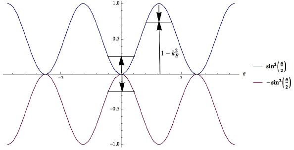
Figure 2. In the figure we show the pendulum potential (blue) for the dynamical motion parameterized with a real time variable. The inverted potential (magenta) corresponds to a dynamics parameterized by a pure imaginary time variable. 

We can solve the equation in two different but equivalent ways: i) the first option consists in writing down the equation in terms of a real time variable and then flipping the sign of the whole equation in order to have positive energies, the resulting equation is of the same form as Eq. (4), ii) the second option consists in solving the equation directly in terms of the imaginary time y. Because both solutions describe to the same physical system, we can conclude that both are just different representations of the same physics. These two-ways of working provide relations between the elliptic functions with different argument and different modulus. As we will discuss the relations among different time variables and modulus can be termed as duality relations and because the mathematical group operation beneath these relations is the S generator of the modular group PSL(2,Z), we can refer to this duality relation as S-duality.

3.3. Equivalent solutions

In the following discussion we will assume without losing generality that 0<k2≤1/2 and therefore that its complementary modulus is defined in the interval 1/2≤kc2<1. The cases where 1/2≤k2<1 and therefore where 0<kc2≤1/2 can be obtained from the case we are considering by interchanging to each other the modulus and the complementary modulus k2↔kc2.

● Oscillatory motion: Let us consider oscillatory solutions for total mechanical energy 0<kE2=k2≤1/2. Solutions for these motions can be expressed in terms of either i) a real time variable and given by Eq. (20), or ii) in terms of a pure imaginary time variable. In the latter case the suitable constant is ỹ0=iK-Kc and according to the Eq. (24) and due to the equivalence of solutions we have

θkx≡2arcsin⁡k snx, k=2 ×arcsin⁡dn ix -iK+Kc, kc≡θkcix. (25)

This result is very interesting, it is telling us that any oscillatory solution can be represented as an elliptic function either of a real time variable or a pure imaginary time variable and although they have the same energy, they differ in the value of its modulus. For solutions with real time the square modulus coincides with the energy kE2 and for solutions with pure imaginary time, the square modulus is equal to 1-kE2. It is clear that the modulus of the two representations of an oscillatory solution satisfies the relation

k2+kc2=1. (26)

As discussed in Appendix B, the elliptic function dn(z, k_c ) has an imaginary period 4iK, therefore the period of the imaginary time oscillatory motion is 4iKg/l, which is in complete agreement with the periods 4Kg/l for the solutions with real time. From Eqs. (25) it is straightforward to compute the angular velocity in terms of an elliptic function whose argument is a pure imaginary time variable (see Table I). A similar result is obtained for an oscillatory motion with energy kE2=kc2.

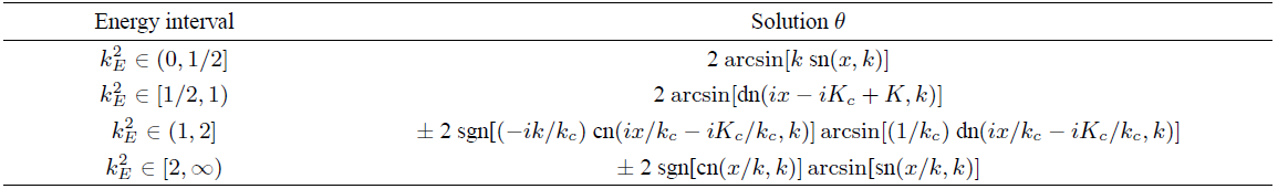
Table I. The third column shows the solutions to the simple pendulum problem in terms of a real time variable when the total mechanic energy of the motion and the square modulus of the Jacobi elliptic function are the same. The fourth column shows its S-dual solutions in terms of a pure imaginary time variable. 

Two final comments are necessary, first in the general solutions (20) and (24) the ± signs appeared, however in (25) there is not reference to them. This happen because they are explicitly necessary only in the circulating motions. In the case of oscillatory motions the (-) sign can be absorbed in the solution by rescaling the time variable in both cases (real and pure imaginary time). Regarding the elliptic function inside the sign function it does not appear because in the case of (20) we have sgn[dn(x, k)] = 1 and also in (24) sgn[k_c sn(ix-iK_c +K, k)] = 1.

● Circulating motion: For the circulating motion we must also separate the energy intervals in two cases. If we are considering the solutions (20) which have real time variable, the corresponding energy intervals are 1<kE2=1/kc2≤2 and 2≤kE2=1/k2<∞. On the other side, if the solution involves a pure imaginary time variable (Eq. (23)) the relevant energies take values in the intervals -1≤1-kE2=-k2/kc2<0, and -∞<1-kE2=-kc2/k2≤-1. Explicitly we have for the first interval

θ1∕kcx≡2 sgn dn x, 1kcarcsin⁡1kc sn x, 1kc=2 sgn i, kkc sn ix-iK, ikkc×arcsin⁡dn ix -iK, ikkc≡θik/kcix. (27)

Notice that in a similar way to the oscillatory case, we have the following relations between the sum of the square modulus

1kc2-k2kc2=1. (28)

Analogous relations can be found for the solutions with energy kE2=1/k2 and for motions in the clockwise direction.

3.4. S group element as member of PSL(2,Z)

It is possible to reach the same conclusions as in the previous subsection but this time following a slightly different path. In Appendix B we have summarized the action of the different group elements of PSL(2,Z) on the Jacobi elliptic functions, in particular the action of the S group element. Starting for instance with a solution involving a real time variable and applying the action of the S group element, it is possible to obtain the corresponding solution in terms of a pure imaginary time variable. As we will show, the obtained results coincide with the ones we have discussed.

● Oscillatory motion: In this case the starting point is the solution (5) and its time derivative (6) which depends on a real time variable and describe an oscillatory pendulum solution with energy kE2. To fix the discussion we choose x ₀ = 0. Applying the Jacobi’s imaginary transformations Eqs. (B.13) which are the transformations generated by the S generator of the PSL(2,Z) group, we obtain

k sn x, k=-ik sc ix, kc=-k ndix +iK, kc=dn ix-iK+Kc, kc (29)

k cn x, k=k nc ix, kc=-ik kc sdix +iK, kc=-ikc cn ix-iK+Kc, kc (30)

recovering relation (25) with their respective expressions for its time derivative. Notice that although the transformed functions have modulus k_c they satisfy

dn2(ix-iK+Kc,kc)-kc2cn2(ix-iK+Kc,kc)=k2, (31)

which is telling that the solution is indeed of oscillatory energy kE2=k2 as it should be. An analogous result is obtained if we start instead with a solution of modulus kc2 and real time variable.

● Circulating case: In the circulating case we have a similar story, under an S transformation the circulating solutions (9)-(10) lead to the set

sgn dn kx, 1k1ksn kx, 1k=sgn ikck sn ix-iK, ikck×dn ix-iK, ikck, (32)

cn kx, 1k=kc cn ix-iK, ikck (33)

which coincide with the solutions (24) for a choice of the constant ỹ0=iK.

4. Web of dualities

4.2 The lattices domain

At this point it is convenient to discuss the domain of the lattices that play a role in the elliptic Jacobi functions and therefore in the solutions of the simple pendulum. As discussed in the Appendix A, the quarter periods of a Jacobi elliptic function whose square modulus is in the interval 0<k2≤1/2, generate vertical lattices represented by a modular parameter of the form τ = iK_c /K. The point τ = i is associated to the case where the rectangular lattice becomes square and corresponds to the value k² = 1/2. The set of all these lattices (black line in Fig. 3) is represented in the complex plane by the left vertical boundary of the region F1 (Fig. 5) since the quotient KcK∈[1,∞). Acting on these values of the modular parameter with the six group elements of PSL(2,Z/2Z) produce the whole set of values of the modular parameter (Fig. 3) that are consistent with the elliptic Jacobi functions. For example, acting with the S group element of Γ on the vertical line τ = iK_c /K, generates the blue vertical line described mathematically by the set of modular parameters τ = iK/K_c , with K/Kc∈(0,1]. It is clear that the set of six lines is a subset of the F2 fundamental region and constitutes the whole lattice domain of the elliptic Jacobi functions.

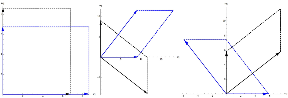
Figure 3. Figure shows the whole domain of values that the modular parameter τ can take for the Jacobi elliptic functions. This domain is a subset of the F2 fundamental region (Fig. 2). Black dots represent the values of the square modulus k² = 1/2, 1 - k² = 1/2, 1/k² = 2, 1/(1 - k²) = 2, 1 - 1/k² = -1 and k²/(k² - 1) = -1. 

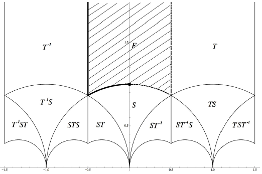
Figure 4. Tessellation of H. The fundamental region F is represented by the shaded area and the heavy part of the boundary. This region is mapped to the whole upper plane C by the modular group Γ. The region can be viewed as a complete list of the inequivalent complex structures on the topological torus since conformal equivalence of tori is determined by the modular equivalence of their period ratios. In the figure we show some copies of the fundamental region obtained by application of some group elements of PSL(2,Z). 

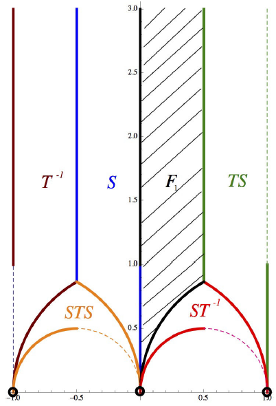
Figure 5. Fundamental cell F2 for Γ(2). The heavy part of the figure is retained, the rest is not. In particular the cusps -1, 0, 1 and iꝏ are excluded. 

In Table II we give the numerical values (approximated) of the generators of the fundamental cell as well as the modular parameter for some values of the square modulus.

Table II. Approximated numerical values of the periods and the modular parameter for some real values of the modulus of the Jacobi elliptic functions. The values k = 0 and k = 1 correspond to limit situations where one of the two periods is lost. The value k² = 1/2 is known as a fixed point, it belongs both to the boundary of the regions F1 and S of the Fig. 5 and is represented by the black dot whose coordinates are (0, i) in Fig. 3. The value k² = 2 is degenerated in the sense it can be represented by two different types of fundamental cells, in one case the cell belongs to the boundary of the region ST S and in the another case it belongs to the boundary of ST^-1. The fundamental cell for some values of k² in this table are plotted in Fig. 6. 

As a conclusion, for every value of the parameter 0<k2≤1/2 there are six normal lattices related one to each other by transformations of the modular group. Therefore each solution of the simple pendulum with real time variable, showed in Table I, can be written in six different but equivalent ways, where each one of the six forms is in one to one correspondence with one of the six normal lattices. Their S-dual solutions (see Table I) which are functions of a pure imaginary time are just one of the six different ways in which solutions can be written.

4.4. A single normal lattice

It is natural to wonder about the minimum number of normal lattices needed to express all the solutions of the simple pendulum. Due to the duality symmetries between lattices this number is one. As an example, if we now use the S-duality to relate the normal horizontal lattice iL^* to the normal vertical lattice L^* , the horizontal lines that compose the domain in the horizontal lattice becomes vertical lines in the vertical lattices, which means to consider solutions with imaginary time in L ^* . Thus we can end up with only one normal lattice and in order to have the four different types of solutions, it is necessary to consider the whole domain of the lattice, i.e. both vertical lines (imaginary time) and horizontal lines (real time) and on each set of lines to consider two different solutions one oscillatory and one circulating. For completeness in Table III we give the four type of solutions in terms of only one value of the modulus.

Table III. Solutions to the simple pendulum problem written in a unique lattice of square modulus 0 < k²≤ 1/2. 

It is clear that we can express all the solutions also for the other five different functional forms of the square modulus.

5. Final remarks

In this paper we have addressed the meaning of the fact that the complex domain of the solutions of the simple pendulum is not unique and in fact they are related by the PSL(2,Z/2Z) group, finding that the important issue for express the solutions is the relation between the values of the square modulus k² of the Jacobi elliptic functions, and the value of the total mechanical energy kE2 of the motion of the pendulum. Due to the symmetry we conclude that there are six different expressions of the square modulus that are related one to each other trough the six group elements of PSL(2,Z/2Z). These six group actions can be termed as duality-transformations and therefore we have six dual representations of k². As a consequence there are six different but equivalent ways in which we can write a specific pendulum solution, and abusing a little bit of the language we could say there are duality relations between solutions. This analysis teach us the lesson that we can restrict the domain of lattices to the ones whose modular parameter is in the pure imaginary interval τ∈i(1,∞), or equivalently that we can express every solution of the simple pendulum either oscillatory or circulating with Jacobi elliptic functions whose value of the square modulus is in the interval 0<k2≤1/2 (see Table III).

It is well known that there are several physical systems in different areas of physics whose solutions are also given by elliptic functions, for instance in classical mechanics some examples are the spherical pendulum, the Duffing oscillator, etc., in Field Theory the Korteweg de Vries equation, the Ising model, etc., ^12,18. It would be very interesting to investigate on similar grounds to the ones followed here, the physical meaning of the symmetries of the elliptic functions in these systems.

References

1. M. R. Matthews, Science Teaching, The role of History and Philosophy of Science (1994). [ Links ]
2. E. T. Whittaker and G. N. Watson, A Course of Modern Analysis (1927). [ Links ]
3. P. Du Val, Elliptic Functions and Elliptic Curves (1973). [ Links ]
4. S. Lang, Elliptic Functions (1973). [ Links ]
5. D. F. Lawden, Elliptic Functions and Applicaions (1989). [ Links ]
6. H. McKean and V. Moll, Elliptic Curves: Function Theory, Geometry, Arithmetic (1999). [ Links ]
7. J. V. Armitage and W. F. Eberlein, Elliptic Functions (2006). [ Links ]
8. P. Appell, Principes de la théorie des fonctions elliptiques et applications (1897). [ Links ]
9. H. Von Helmholtz and O. Krigar-Menzel, Die Dynamik Discreter Massenpunkte (1898). [ Links ]
10. E. T. Whittaker, A treatise on the Analytical Dynamics of particles and Rigid Motion (1917). [ Links ]
11. A. Beléndez, C. Pascual, D. I. Méndez, T. Beléndez, and C. Neipp, Rev. Bras. Ensino Fis. 29 (2007) 645. [ Links ]
12. A. J. Brizard, Eur. J. Phys. 30 (2009) 0711-4064. [ Links ]
13. K. Ochs, Eur. J. Phys. 32 (2011) 479. [ Links ]
14. N. C. Abel, Journ. fur Math. 2 (1827) 101. [ Links ]
15. C. G. J. Jacobi, Astronomische Nachrichten 6 (1827) 133. [ Links ]
16. C. G. J. Jacobi, Fundamenta Nova Theoriae Functionum Ellipticarum (1829). [ Links ]
17. F. Klein, Vorlesungen über die Theorie der elliptischen Modulfunktionen (1890). [ Links ]
18. P. M. Petropoulos and P. Vanhove (2012) 1206-0571. [ Links ]
19. J. H. Schwarz, Nucl. Phys. Proc. Suppl. B 55 (1997) 1. hep-th/9607201. [ Links ]
20. C. P. Burgess and B. P. Dolan, Phys. Rev. B 63 (2001) 155309. hep-th/0010246. [ Links ]
21. P. Appell, Comptes Rendus Hebdomadaires des Scances de l’Acadmie des Sciences 87 (1878). [ Links ]
22. J. P. Serre, A Course in Arithmetic (1973). [ Links ]
23. F. Diamond and J. Shurman, A First Course in Modular Forms (2000). [ Links ]
24. M. Nakahara, Geometry, topology and physics (2003). [ Links ]
25. L. E. Reichl , The Transition to Chaos, In Conservative Classical systems: Quantum Manifestations (1992). [ Links ]
26. M. Lara and S. Ferrer, European Journal of Physics 36 (2015) 055040. [ Links ]
27 This map can be interpreted as a canonical transformation see e.g.25,26
28 Be aware that we are following the mathematics literature in which often it is referred with the same name fundamental region, to two different kind of regions, the one that we have denoted as FN and the one just described. We expect do not generate confusion.
Appendix
A. The modular group and its congruence subgroups
A.1 The modular group
The modular group Γ is the group defined by the linear fractional transformations on the modular parameterτC (see for instance 3,4,5,6,7,22,23 and references therein)
τΓ(τ)=aτ+bcτ+d, (A.1)
where a,b,c,dZ satisfying ad - bc = 1, and the group operation is function composition. These maps all transform the real axis of the τ plane (including the point at infinity) into itself, and rational values into rational values. The group has two generators defined by the transformations
S(τ)-1/τ,     and       T(τ)1+τ. (A.2)
The modular group is isomorphic to the projective special linear group PSL(2,Z), which is the quotient of the 2-dimensional special linear group SL(2,Z) by its center {I,-I}. In other words, PSL(2,Z)=SL(2,Z)/Z2 consists of all matrices of the form
A=abcd, (A.3)
with unit determinant, and pair of matrices A, -A, are considered to be identical. The group operation is multiplication of matrices and the generators accordingly with (A.2) are
S=0-110,    T=(1101). (A.4)
These group elements satisfy S2=(ST)3=-II and Tn=1n01.
One important property of the modular group is that the upper half plane of C, usually denoted as H and defined as H{zC:Im(z)>0}, can be generated by the elements of PSL(2,Z) from a fundamental domain or regionF. Mathematically this region is the quotient space F=H/PSL(2,Z) and satisfies two properties: (i) F is a connected open subset of H such that no two points in F are related by a Γ transformation (A.1) and (ii) for every point in H there is a group element gΓ such that gτF. There are many ways of constructing F, and the most common one found in the literature is to take the set of all points z in the open region {z:-1/2<Re(z)<1/2|z|>1}, union “half” of its boundary, for instance, the one that includes the points: z = -1/2 + iy with ysin(2π/3), and |z| = 1 with -1/2Re (z)0 (see Fig. 4). It is assumed that the imaginary infinite is also included.
Geometrically, T represents a shift of F to the right by 1, while S represents the inversion of F about the unit circle followed by reflection about the imaginary axis. As an example, the Fig. 4 represents the transformations of the fundamental region F by the elements of the group: {I, T, T-1, S, TS, T-1S, ST, ST-1,ST-1S, TST-1, STS,T-1ST} 22. Notice that these 12 elements are all the independent ones that we can construct as iterative products of S, T and T -1 without powers of any of them involved (S -1 is simply -S ~ S and therefore is not a different modular transformation). The other two transformations we can construct are not independent TST = -ST -1 S and T -1 ST -1 = STS -1. Further products of the generators with these transformations give us the whole tessellation of the upper complex plane. In particular the orbit of the points Im(z)→ꝏ are the rational numbers Q and are called cusps.
A.2 Congruence subgroups
Relevant for our discussion are the congruence subgroups of level N denoted as Γ(N) (or Γ N ). They are defined as subgroups of the modular group Γ, which are obtained by imposing that the set of all modular transformations be congruent to the identity mod N
ΓN=abcdSL2,Z : abcd=1001mod N. (A.5)
In this nomenclature the modular group Γ is called the modular group of level 1 and denoted as Γ(1) 6,23. A relevant mathematical structure is the coset of the modular group with the congruence subgroups which are isomorphic to PSL(2,Z/NZ) 23
SL(2,Z)Γ(N)PSL(2,Z/NZ). (A.6)
For the solutions of the simple pendulum the relevant congruence subgroup is the one of level 2: Γ(2). It turns out that all the groups PSL(2,Z/NZ) are of finite order and in particular PSL(2,Z/2Z) is of order six. In Table IV we give explicitly the six elements of the coset and their corresponding form as group elements of PSL(2,Z). Analogously to the case of the modular group, a fundamental cell for a subgroup Γ(N) is a region FN in the upper half plane that meets each orbit of Γ(N) in a single point. Because Γ(2) is of order six in Γ, a fundamental cell for Γ(2) can be formed from the six copies of any fundamental cell F of Γ produced by the action of the six elements. In Fig. 5 we show the fundamental region F2 of Γ(2). This cell can be obtained from the region denoted as F1 which is a different fundamental region for Γ as compared to the usual region F of the Fig. 4. F1 is obtained if F is replaced by its right half, plus inversion of its left half by the S transformation. Thus F1 consists of the open region {z:0<Re(z)<1/2(zz¯/z+z¯)>1} and part of its boundary must be included. Geometrically (zz¯/z+z¯)=1 represents a unitary circle with centerat z = 1. A possible choice of the boundary includes the set of all points z:z=iy with y1 union {z:(zz¯/z+z¯)=1 with 0< Re (z)1/2} . The full fundamental region F2 so produced is the part of the half-plane above the two circles of radius 1/2 centered at ±1/2.
Table IV. Main characteristics of the six order PSL(2,Z/2Z) group and its relation to the six normal lattices.
As a complementary comment we mention that sometimes in the literature Γ(2) appears under the name of modular groupΛ. It turns out that the group is isomorphic to the symmetric group S 3, which is the group of all permutations of a three-element set and also to the dihedral group of order six (degree three) D 6, which represents, the group of symmetries (rotations and reflections) of the equilateral triangle.
A.3 Lattices
A lattice L is an aggregate of complex numbers with two properties 3: (i) is a group with respect to addition and (ii) the absolute magnitudes of the non-zero elements are bounded below. Because the Jacobi elliptic functions are meromorphic functions on C, that are periodic in two directions: f(z)=f(z+ω1)=f(z+ω2), we are interested in the so-called double lattices, consisting of all linear combinations with integer coefficients of two generating coefficients or primitive periodsω1,ω2C, whose ratio is imaginary
L(ω1,ω2)=nω1+mω2n,mZ   such that   f(z)=fz+nω1+mω2,  zC. (A.7)
The lattice points are the vertices of a pattern of parallelograms filling the whole plane, whose sides can be taken to be any pair of generators. The shapes of the lattices define equivalence classes. If L(ω1,ω2) is any lattice, and the number k0C, then kL(ω1,ω2) denotes the aggregate of complex numbers kz for all zL(ω1,ω2) and it is also a lattice, which is said to be in the same equivalence class as L(ω1,ω2). If L¯ denotes the aggregate of complex numbers z¯,  zL; L¯ is also a lattice. If L¯=L, the lattice is called real. If the primitive periods can be chosen so that ω 1 is real and ω 2 pure imaginary, L is called rectangular.
Rectangular lattices are real, and they are called horizontal or vertical, according as the longer sides of the rectangles are horizontal or vertical. The particular case in which both sides are equal is called the square lattice. Every lattice satisfies L = -L, and the only square lattice for which, L = αL, with α±1, is the lattice iL. If L is a vertical rectangular lattice, iL is a horizontal rectangular lattice and vice versa.
Associated to the lattice is the concept of residue classes. If z is any complex variable, z + L denotes the aggregate of values z + ω for all ω in the lattice L. This aggregate is called a residue class (mod L). The residue classes (mod L) form a continuous group under addition, defined in the way (z+L)+(w+L)=(z+w)+L. L itself is a residue class (mod L), the zero element of the group. These residue classes allow to introduce the concept of fundamental region of L, consisting in a simply connected region of the complex plane which contains exactly one member of each residue class (mod L) 28. A fundamental region can be chosen in many ways, the simplest and usually the most convenient, is what is called either a unit cell, a fundamental cell or a fundamental parallelogram which is defined by all the points of the sides ω1 and ω2, including the vertex 0, but excluding the rest of the boundary and of course the whole interior points of the parallelogram. Mathematically the cell is given by the coset space C/L(ω1,ω2), where abusing of the notation, in this expression L is considered as a residue class. Since the opposite sides of the fundamental cell must be identified, the coset space C/L(ω1,ω2) is homeomorphic to the torus T2. In other words, the pair (ω 1, ω 2) defines a complex structure of T2 24.
The shape of the lattice is determined by the modular parameterτω2/ω1. It is important to note that, while a pair of primitive periods ω 1, ω 2, generates a lattice, a lattice does not have any unique pair of primitive periods, that is, many fundamental pairs (in fact, an infinite number) correspond to the same lattice. Specifically a change of generators ω1, ω2 to ω1' and ω2' of the form
ω2'ω1'=abcdω2ω1, (A.8)
induces a mapping on the modular parameter τ, belonging to the modular group. These maps are the link between the concepts of lattices, torus and modular group. As an example we discuss the mapping on τ induced by the generators (A.2). The generator S interchanges the roles of the generators of the lattice ω1ω2 or equivalently it changes the longitude l for the meridian m of the torus and vice versa. The transformation T generates a Dehn twist along the meridian which can be understood as follows 24. As a first step cut the torus along the meridian m, then take one of the lips of the cut and rotate it by 2π with the other lip kept fix and finally glue the lips together again.
If the stationary values e1, e2 and e3 are the roots of the cubic equation 4x3-g2x-g3=0, for any lattice L, with assigned generators ω1, ω2, we can define the scale constant h by means of the relation: h2 = e1 - e2, and the moduli as
k2=e3-e2h2,  kc2=e1-e3h2. (A.9)
A lattice for which h2 = 1 is called normal, and using the notation of 3, we write it with a star L* . Every lattice L with assigned generators is similar to a unique normal lattice L* =hL with corresponding generators, since ei(hL)=h-2ei(L). For a given lattice shape with no assignments of generators, there are six normal lattices, as any of the six differences ei - ej , can be taken as h2. If one of these is L* , with modulus k, the others are iL* , kL*, ikL* , kcL* and ikcL*, with moduli kc , 1/k, ikc /k, ik/kc and 1/kc respectively, where k2+kc2=1. These fall into three pairs which are of the same size, interchanged by a rotation of a right angle.
For the rectangular lattice shape, the six normal lattices are all real. Ordinarily ω1 is taken real and ω2 pure imaginary, so that e1 > e3 > e2, and 0<k2<1, 0<kc2<1 with k2<1/2<kc2 if L is vertical. We summarize the properties of the normal lattices in table.
Figure 6. Figure shows the fundamental cell for six different normal lattices. In the first plot the vertical cell corresponds to a value of the square modulus k 2 = 1/4 and belongs to a normal lattice of the type L * . Under an S transformation, the cell transforms to the horizontal one whose value of the square modulus is k 2 = 3/4 and belongs to a normal lattice iL * . Analogously in the second and third plots, the fundamental cells in black belong to the lattices kL * and i c kL * respectively, with values of the square modulus k 2 = 4 and k 2 = 4/3. The blue cells are obtained as their S-dual fundamental cells and have the values k 2 = -3 and k 2 = -1/3 and belong to normal lattices of the kind ikL * and k c L * respectively. In every case, the continuous lines are included in the fundamental cell, whereas the dashed lines are not. The numerical values of the two generators ω 1 and ω 2 are given in table.
B. Jacobi elliptic functions
In the previous appendix we reviewed the action of the modular group on the modular parameter. In this appendix we want to specialize that discussion to the case of the elliptic Jacobi functions. In particular we are interested in the relation between the six dimensional group PSL(2,Z/2Z) and what is called transformations of the elliptic Jacobi functions. There are three transformations that are exposed often in the literature, the Jacobi’s imaginary transformation, the Jacobi’s imaginary modulus transformation and the Jacobi’s real transformation. These are transformations that relate the Jacobi elliptic functions with different value of the square modulus k 2. Behind these transformations is the property that the modulus of the Jacobi functions can be defined in the real line k2R with exception of the points z = -1, 0, 1, and it can be divided in six intervals
k2-,-1-1,00,1212,11,2[2,).
These six intervals are in one to one relation to the column Action on k 2 in Table IV, if we consider that the modulus in the fundamental region F1 of PSL(2,Z) takes values in the interval 0k21/2. In the following we summarize some of the properties of the Jacobi elliptic functions that are useful throughout the paper.
B.1 Jacobi elliptic functions with modulus 0 < k2 < 1
The Jacobi elliptic functions are meromorphic functions in C, that have a fundamental real period and a fundamental complex period, i.e., they are doubly periodic. The periods are determined by the value of the square modulus and in the following we assume that 0 < k2 < 1.
The primitive real period of the three basic functions can be inferred from the following relations which are dictated by the addition formulas for the Jacobi functions 2,3,4,5,6,7
sn(z+K,k)=cn(z,k)dn(z,k),        cnz+K,k=-kcsnz,kdnz,k,            dn(z+K,k)=kc1dn(z,k), (B.1)
where the quarter-period K is defined as function of the square modulus k2 as
K01du(1-u2)(1-k2u2). (B.2)
In particular we obtain the values sn(K, k) = 1, cn(K, k) = 0 and dn(K, k) = k c , from the ones (0, k) = 0, (0, k) = 1 and (0, k) = 1. Iteration of relations (B.1) leads to
sn(z+2K,k)=-snz,k,    cnz+2K,k=-cnz,k,    dn(z+2K,k)=dn(z,k). (B.3)
The last relation is telling that the function dn(z, k) has real period 2K. A further 2K iteration will tell us that the other two Jacobi elliptic functions (sn(z, k) and cn(z, k)) have primitive real period 4K. Regarding the complex period, we have the relations
sn(z+iKc,k)=1k1sn(z,k),     cn(z+iKc,k)=-i1kdnz,ksnz,k,     dn(z+iKc,k)=-icn(z,k)sn(z,k), (B.4)
Where Kc is defined as function of the so-called complementary modulus kc21-k2 in the form
Kc01du(1-u2)(1-kc2u2). (B.5)
Iterating these relations once leads to
sn(z+2iKc,k)=snz,k,         cnz+2iKc,k=-cnz,k,      dn(z+2iKc,k)=-dn(z,k). (B.6)
The first relation is telling us that the elliptic function sn(z, k) has a pure imaginary primitive period 2iK c . A further 2iK c iteration leads to the conclusion that the elliptic function dn(z, k) has a pure imaginary primitive period 4iK c whereas the elliptic function cn(z, k) has a fundamental period 4iK c . In the latter case notice that combining the second relation of (B.3) and the second relation of (B.6) leads to the result cn(z + 2K + 2iK c , k) = cn(z, k) concluding that this elliptic function has a primitive complex period 2K + 2iK c .
In summary, the primitive periods of the three basic Jacobi functions are
sn(z,k)=sn(z+4K,k)=sn(z+2iKc,k), (B.7)
cn(z,k)=cn(z+4K,k)=cn(z+2K+2iKc,k), (B.8)
dn(z,k)=dn(z+2K,k)=dn(z+4iKc,k). (B.9)
Because these periods do not coincide one looks for two common periods in order to define a common fundamental cell for the three functions. These fundamental periods are 4K and 4iK c , they are not primitive because linear combinations of them does not give origin for instance to the primitive period 2K + 2iK c of cn(z, k). The fundamental cell for the Jacobi elliptic functions is, therefore, the parallelogram with vertices (0, 4K, 4iK c , 4K + 4iK c ), and the modular parameter τ turns out to be
τiKcK. (B.10)
Given this definition of the modular parameter we see that not every point of F1 corresponds to a modulus k 2 of the Jacobi functions but only the values on the vertical boundary τ[i,i), being the point τ = i the one that corresponds to k 2 = 1/2, since in this case K = K c and therefore the corresponding normal lattice is squared. The rest of points on the vertical boundary corresponds to vertical normal lattices because K < K c and all of them have a value of the square modulus 0 < k 2 < 1/2. By acting the five group elements of PSL(2,Z/2Z) different from the identity to the modular parameter values on the vertical boundary of F1, we can generate the whole set of possible values of τ and therefore the whole set of possible values of the square modulus k 2 of the Jacobi functions (see Fig. 3).
Derivatives of the basic functions, which are necessary to obtain the angular velocities are
ddzsn(z,k)=cnz,k  dnz,k,           ddzcn(z,k)=-snz,k dnz,k,       ddzdn(z,k)=-k2sn(z,k)cn(z,k). (B.11)
B.2 Jacobi’s imaginary transformation
The transformation induced by the generator S(τ) of the modular group on the Jacobi functions with modulus k, is known as the Jacobi’s imaginary transformation. In this case the modulus and the complementary modulus exchange with each other
kkcand        kckKKcand             KcK. (B.12)
Applying this transformation on the vertical boundary of F1, generates both the transformed pure imaginary modular parameter and the transformed modulus which belong to the intervals τ(0,i] and 1/2kc2=1-k2<1, respectively. The Jacobi functions itself transform as
sn(z,kc)=-isciz,k,          cnz,kc=nciz,k,              dn(z,kc)=dc(iz,k). (B.13)
This is the mathematical property behind the analysis made by Appell to deal with solutions of imaginary time. These transformations are used very often to change a pure imaginary argument ix to one real x, obtaining
sn(ix,k)=i  scx,kc,        cnix,k=ncx,kc,          dn(ix,k)=dc(x,kc). (B.14)
From a geometrical point of view the normal vertical cell L * with vertices (0,4K, 4iK c , 4K + 4iK c ) changes to the normal horizontal cell iL * with vertices (0,4K c , 4iK, 4K c + 4iK) and the corresponding torus is obtained from the original one by an interchange of their respective meridians and longitudes. The rest of properties of the functions are obtained from the ones in (section) by setting z = ix and implementing in the expressions the interchanges kkc and KKc.
B.3 Jacobi’s imaginary modulus transformation
The transformation induced by the generator T(τ) of the modular group on the Jacobi functions, is known as the imaginary modulus transformation, because under this transformation the modulus change as
kikkc,          and               kc1kc, (B.15)
which induces a change in the quarter periods of the form
KkcK,         and              Kckc(Kc-iK). (B.16)
Applying this transformation to the vertical boundary of F1, generates the transformed modular parameter which lies on the vertical line τ[1+i,1+i) and the transformed square modulus which takes values in the interval -1(k2/k2-1)<0. The transformation rule for the Jacobi functions itself are
sn(z,ik/kc)=kcsd(z/kc,k),               cn(z,ik/kc)=cdzkc,k,                       dn(z,ik/kc)=nd(z/kc,k). (B.17)
It is clear that this transformation allows us to define the Jacobi functions with an imaginary modulus in terms of the Jacobi functions with real modulus. Replacing zkcz, we can express these transformations in its more usual form
sn(kcz,ik/kc)=kcsdz,k,                   cn(kcz,ik/kc)=cdz,k,                  dn(kcz,ik/kc)=nd(z,k). (B.18)
From a geometrical point of view the fundamental vertical cell with vertices (0,4K, 4iKc , 4K + 4iKc ) changes to the fundamental cell with vertices (0,4kc K, 4kcK, + 4iKcK, 8kcK + 4ikcKc ) and the corresponding torus is changed by a Dehn twist. Notice that by applying further the transformation S to these expressions, we obtain a fundamental cell where the quarter periods (B.16) are interchange among them an the value of the square modulus is defined in the interval, 1<(1/1-k2)2, since the modulus (B.15) also interchanges one to the another.
The elliptic Jacobi functions with negative square modulus satisfy analogous relations to the Jacobi functions with modulus 0 < k2 < 1, these are obtained from Eqs. (B.17) and the corresponding relation of the Jacobi functions with 0 < k2 < 1. For instance, the equations analogous to (13) and (15) are
sn2(z,ik/kc)+cn2(z,ik/kc)=1,               and-k2kc2sn2(z,ik/kc)+dn2(z,ik/kc)=1. (B.19)
Proceeding in a similar way it is possible to obtain the equations analogous to (B.1), these are
sn(z+K,ik/kc)=cn(z,ik/kc)dn(kcz,ik/kc),             cn(z+K,ik/kc)=-1kcsn(z,ik/kc)dn(kcz,ik/kc),                  dn(z+K,ik/kc)=1kc1dn(z,ik/kc), (B.20)
which iterating once lead to the relations
sn(z+2K,ik/kc)=-sn(z,ik/kc),                    cn(z+2K,ik/kc)=-cn(z,ik/kc),                    dn(z+2K,ik/kc)=dn(z,ik/kc). (B.21)
The third relation is telling us that the function dn(z, ik/kc ) has a fundamental period 2K. A further 2K iteration leads to the conclusion that the other two Jacobi functions have a fundamental period of 4K. Regarding the imaginary period, the equations analogous to (B.4) are
sn(z+iKc,ik/kc)=ikckdn(z,ik/kc)cn(kcz,ik/kc), (B.22)
cn(z+iKc,ik/kc)=1k1cn(z,ik/kc), (B.23)
dn(z+iKc,ik/kc)=i1kcsn(z,ik/kc)cn(kcz,ik/kc), (B.24)
which after an iteration lead to
sn(z+2iKc,ik/kc)=-sn(z,ik/kc),                     cn(z+2iKc,ik/kc)=cn(z,ik/kc),                      dn(z+2iKc,ik/kc)=-dn(z,ik/kc). (B.25)
These relations indicate that the function cn(z, ik/kc ) has fundamental imaginary period 2iKc , whereas the other two Jacobi functions have 4iKc . In summary, the primitive periods of the three basic Jacobi functions are
snz, ikkc=snz+4K, ikkc=sn z+2K+2iKc, ikkc, (B.26)
cnz, ikkc=cnz+4K, ikkc=cn z+2iKc, ikkc, (B.27)
dnz, ikkc=dnz+2K, ikkc=dn z+4iKc, ikkc, (B.28)
It is straightforward to verify that in this case the derivatives of the fundamental relations that follows from (B.11) are
ddzsn(z,ik/kc)=cn(z,ik/kc)dn(z,ik/kc),                    ddzcn(z,ik/kc)=-sn(z,ik/kc)dn(z,ik/kc), (B.29)
and
ddzdn(z,ik/kc)=k2kc2sn(z,ik/kc)cn(z,ik/kc). (B.30)
B.4 Jacobi’s real transformation
In the literature of the elliptic functions, the transformation generated by the element ST S of the modular group
τI=τ1-τ, (B.31)
which can be obtained as a composition of the following three transformations
τI=-1τ2,           τ2=1+τ1,          and       τ1=-1τ,   (B.32)
generates the so-called Jacobi’s real transformation. Under it, the modulus of the elliptic functions change as
k1k,   and  kcikck, (B.33)
whereas the quarter periods transform as
KkK-iKc,          and               KckKc. (B.34)
Applying this transformation to the vertical boundary of F1, generates the transformed modular parameter which lies on the line τ=-(y2/1+y2)+i(y/1+y2), with y in the interval y[1,) and the transformed square modulus which takes values in the interval 21/k2<. The transformation rules for the Jacobi functions itself are
sn(z,1/k)=k        sn(z/k,k),                    cn(z,1/k)=dn(z/k,k),              dn(z,1/k)=cn(z/k,k). (B.35)
This transformations allows us to define the Jacobi elliptic functions with square modulus greater than two in terms of Jacobi functions with modulus 0<k21/2. Replacing zkz, allows to express these transformations in its more usual form
sn(kz,1/k)=k     snz,k,            cn(kz,1/k)=dn(z,k),          dn(kz,1/k)=cn(z,k). (B.36)
A further application of the group transformation S to these expressions leads to the interchange of the modulus (B.33) and to the interchange of the quarter periods (B.34). In this case the square modulus of the Jacobi functions is defined in the interval -<1-1/k2-1.
As in the previous cases it is possible to obtain the fundamental periods of the three different basic Jacobi elliptic functions, since the arguments as before, we just list the equations. For the real period we have
sn(z+K,1/k)=kdn(z,1/k)cn(z,1/k),                 cn(z+K,1/k)=kc1cn(z,1/k),                    dn(z+K,1/k)=-kcksn(z,1/k)cn(z,1/k), (B.37)
and iterating we get
sn(z+2K,1/k)=-sn(z,1/k),              cn(z+2K,1/k)=cn(z,1/k),                        dn(z+2K,1/k)=-dn(z,1/k). (B.38)
As for the imaginary period
sn(z+iKc,1/k)=ksn(z,1/k),                    cn(z+iKc,1/k)=-ikdn(z,1/k)sn(z,1/k),                       dn(z+iKc,1/k)=-icn(z,1/k)sn(z,1/k), (B.39)
and after an iteration
sn(z+2iKc,1/k)=sn(z,1/k),                   cn(z+2iKc,1/k)=-cn(z,1/k),                      dn(z+2iKc,1/k)=-dn(z,1/k). (B.40)
snz, 1 k=sn z+4K, 1k=snz+2iKc, 1k (B.41)
cnz, 1 k=cn z+2K, 1 k=cnz+4iKc, 1k (B.42)
dnz, 1 k=dn z+4K, 1 k=dnz+2K +2iKc, 1k (B.43)
Finally, the equations analogous to (13) and (15) are
sn2z, 1k+cn2z, 1k=1,      and      1k2sn2z, 1k+dn2z, 1k=1. (B.44)
whereas the derivatives of the basic functions are
ddzsn(z,1/k)=cn(z,1/k)dn(z,1/k),                ddzcn(z,1/k)=-sn(z,1/k)dn(z,1/k), (B.45)
ddzdn(z,1/k)=-1k2sn(z,1/k)cn(z,1/k). (B.46)
Received: September 11, 2017; Accepted: January 16, 2018
Creative Commons License This is an open-access article distributed under the terms of the Creative Commons Attribution License