


 text new page (beta)
 English (pdf)
 Article in xml format
 Article references
 Send this article by e-mail
 Cited by SciELO
  Similars in
SciELO
Similars in
SciELO 
 Permalink
PACS: 42.55.Wd; 42.65.Re.
1. Introduction
A mode-locked fiber laser (ML-FL) is a device that is able to produce short and ultra-short optical pulses (ns and fs-ps). This kind of pulse finds applications in pressure sensors 1,2, gas sensors 3, micromachining of materials 4, and supercontinuum generation 5,6, among others. However, there are many implicit effects in the formation and generation of ultra-short pulses, which possibly limit their use for some specific applications. For this reason, the study of the generation and dynamics of ultra-short pulses in a ML-FL remains a hot research topic.
To achieve pulsed operation, we can use for instance the mode locking technique. It divides into two categories: the first one is passive mode locking 7,8,9, which relies on a mechanism of modulation of cavity losses that operates by itself, without external intervention; the second one is active mode locking10,11, which uses an externally driven acousto-optic or electro-optic element that produces a controlled modulation of losses in time.
In a passively mode-locked fiber laser (PML-FL), the gain medium and saturable absorber (SA) initiate the pulsing operation. The SA is an optical device that functions as a nonlinear filter which absorbs low-power radiation and transmits high-power component of a signal. The SA can be classified in function of their saturation time; when the time response of the SA is shorter than the pulse duration, it is known as fast saturable absorber (FSA) 12,13,14; when its time response is longer, it is known as slow saturable absorber (SSA) 15,16.
Commonly, for introducing a power-selective loss, PML-FLs include a physical SA, like the semiconductor saturable absorber mirror (SESAM) 16, 17 18, the most commonly used, although the SESAM has the inconvenient that it usually generates pulses with low energy. Besides, quantum dots embedded in a semiconductor material are used as SA in ML-FLs 19,20 generating low saturation fluence. On the other hand, physical SAs have also been implemented from carbon nanotubes21,22, with which high pulse repetition rates can be generated in a compact cavity. Besides, graphene SAs have been implemented in femtosecond pulse generation23,24.
Other PML-FLs have a figure-eight or ring configuration; for these architectures, usually an artificial SA is used, which relies on non-linear effects generated in optical fiber, so indirectly the absorbed energy through to a laser component (commonly a polarizer or an isolator) is reduced by the changes that produces the non-linear effect. The Non-linear Optical Loop Mirror (NOLM) 6,25,26, the Non-linear Amplifying Loop Mirror (NALM) 28,35 or the Non-linear Polarization Rotation (NPR) 9,29 effect are examples of artificial SA implemented in PML-FLs. Commonly, the NPR effect is the SA meachanism used in a passively mode-locked fiber ring laser (PML-FRL); the latter is studied in this paper.
In recent years, the dynamics of pulses generated by ML-FL have been studied with experimental analysis and theoretical models. Different behaviors and interactions of pulses have been investigated, which encompass different types of pulses: noise-like pulses (NLPs) 6,25,26,28, dissipative solitons 30,31, spiny solitons 32, among others. A recently developed tool, which is useful in ML-FL researches, is a 3D mapping technique of the pulse temporal profile, which helps analyzing pulse dynamics 31,33,34,35,36.
In this paper, we implement a theoretical analysis of the 3D mapping of a pulse conglomerate and of a single pulse (shorter-wavelength component and longer-wavelength component, respectively) in anomalous and normal dispersion regimes of a ML-FL. This study helps us to interpret the 3D mapping measurements in terms of pulse dynamics. Besides, an example of experimental 3D mapping measurement is presented in the case of a regime where a NLP coexists with bunches of solitons generated by a PML-FRL.
2. Theoretical model of the mode-locking by the superposition principle of the electric field
One of the most common models to explain the generation of short pulses by mode-locking will be presented 37. Mode locking means that all modes propagating in the optical fiber resonator are locked in phase; in a model of 2n + 1 modes with the same amplitude E 0, the mode-locking is imposed by the condition of constant phase between two consecutive modes, written as
where:
where the difference in frequency between 2 consecutive modes is constant
where:
The amplitude A(t) is simplified by the geometrical progression given by
where in this case
The total electric field at the output laser is represented as
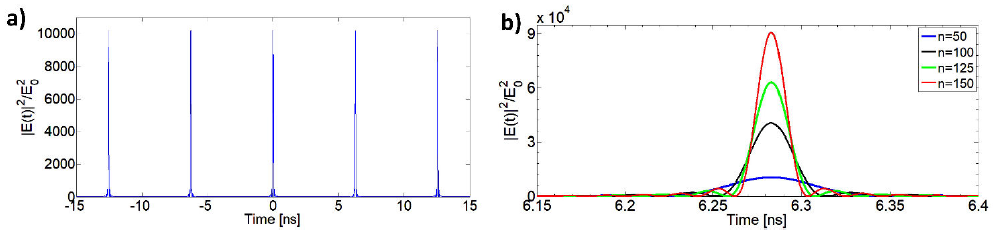
and its mathematical structure is the result of imposing the condition of mode-locking (all modes are in phase or locked); so it is expected that the field intensity I = |E(t)|2 is a periodic train of pulses, as shown in Fig. 1a, which plots the dimensionless intensity (
3. The operation principles in a PML-FRL
The operation of a fiber ring laser (FRL) with passive mode locking is possible thanks to the use of specific optical elements and non-linear effects; these will be explained in this Section.
All lasers consist of three main parts: a gain medium, an external pumping, and a resonant cavity; the latter makes possible the laser beam emission; in the present case, the cavity is a fiber ring. The resonance mechanism in the FRL starts with an initial signal, generated in the cavity, which is amplified at each round-trip until its energy remains stable. The basic elements in a PML-FRL are shown in Fig. 2, the cavity consists of a SA, a gain medium, the chromatic dispersion effect (introduced by the fiber), a polarization controller, an optical isolator (which allows the beam propagation to be unidirectional), output coupler and the nonlinear optical effects (also produced by the fiber).

The gain medium, in turn, consists of an optical fiber doped with a rare-earth element (the most common doped fiber used in communications is the erbium-doped fiber (EDF) 38) fed by an optical pump, which in this case can be a laser diode coupled with the doped fiber; the laser diode emits at a wavelength at which the ions of the doped fiber present strong absortion.
The chromatic dispersion is an effect that occurs in a transparent medium, in this case, a silica optical fiber. This effect causes the phase velocity and the group velocity of the light propagating in fiber to be dependent on the optical frequency 39. The origin of chromatic dispersion is the variation of the refractive index as a function of the wavelength of light. The most usual and economic form to introduce chromatic dispersion in the ring cavity is by inserting several meters of standard single mode fiber (SMF). This type of fiber will introduce anomalous chromatic dispersion; this kind of dispersion causes the refraction index to increase if the wavelength increases; in other words, the longer-wavelength components travel slower with respect to the shorter-wavelength components. On the other hand, it is possible to use dispersion compensating fiber, which introduces normal dispersion in the PML-FRL; this means that the longer-wavelength components travel in this case faster than the shorter-wavelengths.
In the context of the nonlinear effects, when the pulse propagates in the optical fiber with high intensity, a phenomenon called the Kerr effect takes place: it produces a dependence of the refractive index as function of the intensity I40 as follows:
where n0 is the refractive index at low-power and n2 is the nonlinear coefficient.
One of the fundamental elements in the ML-FL is the SA, introduced in the first Section. Its action is that of a nonlinear filter that absorbs the low-intensity components of a signal, and transmits the high-intensity components, which are able to saturate the device; for this reason, the SA favors the generation of short or ultrashort pulses by the laser.
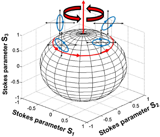
The SA in the PML-FRL is produced through the effect of the non-linear polarization rotation (NPR) and the use of a linear polarizer inserted in the cavity. The SA principle is explained by the scheme in Fig. 3, first an elliptical polarization state is imposed; this condition can be achieved with the polarization controller (array of polarizers and wave retarder plates). In the first case, at low power (Fig. 3a), the elliptical polarization state does not undergo NPR, this means that the initial polarization state does not change during propagation; besides, if its major axis is orthogonal to the polarizer axis, then the transmission is nearly zero. In the second case, at high powers (Fig. 3b), the components of the elliptical polarization state propagating in the fiber induce a nonlinear birefringence; the latter will cause the elliptical polarization state to rotate as it propagates: this is the essence of the NPR effect 41. One way to visualize NPR is using the representation of the Stokes vector on the Poincare sphere; NPR corresponds to a rotation around axis S342, as shown in Fig. 4.
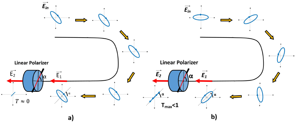
Figure 3. Scheme of the SA mechanism by the NPR in elliptical polarization state and linear polarizer: a) low-powers (without the NPR, there is no SA effect). b) high-powers (with the NPR there is a SA effect).
So, recapitulating the scheme of Fig. 3b, the main idea of the SA (nonlinear filter) is that the elliptical polarization state crosses the linear polarizer, hence the transmission is maximum when the major axis of the ellipse is aligned with the orientation of the polarizer (which occurs at high power, due to NPR), and is minimal if the major axis is perpendicular to the polarizer (at low power, when no NPR takes pace). Hence, the transmission through the linear polarizer depends on the power of the incident beam.
The saturable absorption effect is analyzed by calculating the transmission through the linear polarizer: T = |E2|2/|E1|2. For this purpose, it is necessary to study the evolution of the polarization state components in the formalism of the Jones vector in a circular polarization base {C+, C-}. The analysis starts with the definition of the Jones vector of the initial polarization state with an initial power P
where 𝜓 is the orientation of the polarization state with respect to the horizontal axis and
u and v are real parameters fulfilling the
condition u2 + v2 = 1, for
an elliptical polarization state
The propagation of the initial polarization state (Eq. (8)) is considered in an ideal case for
an isotropic fiber of length L. The contribution of the nonlinear phase is
The polarization state E1 passes through the linear polarizer; the latter is oriented with an angle α with respect to the horizontal axis. Hence, at the output of the polarizer, the following polarization state E2 is obtained
with the transformation matrix of the linear polarizer, we have
Finally, the mathematical expression of the linear polarizer transmission is given by
In Eq. (12), a dependence of the NPR appears associated with the term
however, in this case, no NPR takes place (r = 0), so that again, the transmission remains constant versus power.
The expression for the transmission of the linear polarizer helps understanding the effect of SA when representing the transmission as a function of the power of the elliptical polarization state (
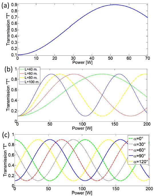
Figure 5. Transmission curve of the linear polarizer considering the NPR of an initial elliptical
polarization state (u = 2 /
which propagates through an isotropic fiber of length L = 100 m with a nonlinear coefficient
with the maximum transmission reached at the critical power
From this expression of the transmission through the linear polarizer aligned with the vertical axis (Eq. 15), it appears that for a longer length L of isotropic fiber a maximum transmission is achieved with a lower power
On the other hand, when considering the same elliptical polarization state and the same
parameters (Ac = 3/5,
4. 3D mapping of the pulse temporal profile
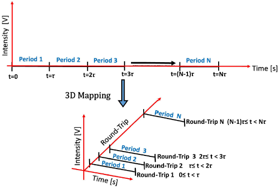
The 3D mapping technique, which is particularly useful to study pulse dynamics, consists of data processing from single-shot sequence measurements of the pulses over N consecutive periods, recorded with a fast oscilloscope, in order to build a 3D sequence of temporal profiles showing the pulses evolution over successive round-trips in the cavity. This temporal profile sequence in 3D is generated by the redistribution of the N consecutive periods (distributed over time) to N consecutive round-trips, as shown in Fig. 6. In this scheme, the consecutive periods are redistributed to consecutive round-trips with a reference system consisting in a short-time axis (covering the duration of the period), a long-time axis (showing the evolution over successive round-trips), and the intensity axis.
The 3D mapping technique is illustrated by the following simulated example. This ideal case presents several pulses, each displaying a soliton envelope (sech2 form); more precisely, there is a pulse conglomerate (five pulses with different peak intensities) that corresponds to shorter-wavelength spectral components and one single pulse that corresponds to longer-wavelength components; consequently, the single pulse and the pulse conglomerate propagate at different velocities. Fig. 7 shows different behaviors in the 3D mapping of this regime. When the ML-FL operates in the anomalous dispersion regime, the single pulse (longer-wavelength components) is delayed with respect to the pulse conglomerate (shorter-wavelength components); in this case the 3D mapping technique presents two behaviors when the single-shot measurement of oscilloscope is triggered on the pulse conglomerate (Fig. 7b) or on the single pulse (Fig. 7c). On the other hand, if the ML-FL operates with normal dispersion, the pulse conglomerate is delayed with respect to the single pulse, Figs. 7d and 7e show the 3D mapping in this case, when the single-shot measurement is triggered on the pulse conglomerate and on the single pulse, respectively.
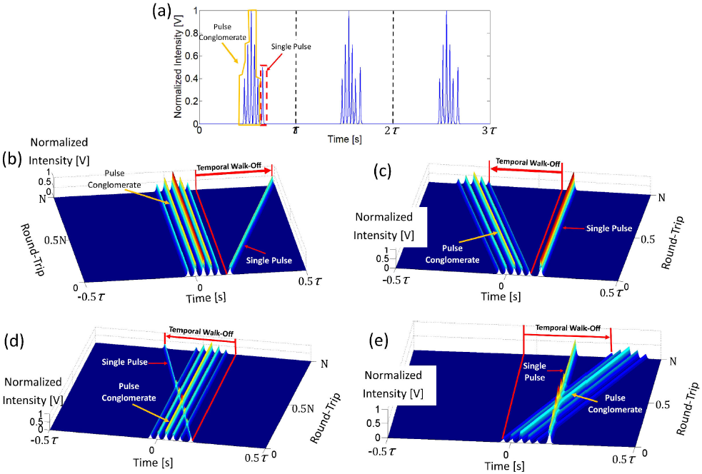
Figure 7. 3D mapping technique applied to characterize the temporal profile (a) of the pulse conglomerate coexisting with the single pulse analyze in anomalous dispersion when the fast oscilloscope trigger is on b) the pulse conglomerate or c) on the single pulse. The other case, in normal dispersion when the fast oscilloscope trigger is on d) the pulse conglomerate or e) the single pulse.
All cases in Fig. 7 show that only one component (pulse
conglomerate or single pulse) has a fixed temporal position over N round-trips,
whereas the other one (single pulse or pulse conglomerate) has a constant temporal
displacement to the right or left, known as temporal walk-off (
4.1. Experimental 3D mapping of a noise-like pulse and bunches of solitons regime generated by a PML-FRL
A regime of noise-like pulse coexisting with bunches of solitons can be achieved in a PML-FRL. The experimental setup (Fig. 8) consists in 20 m of optical fiber in a ring configuration: 1 m of erbium-doped fiber (EDF, Liekki ER30-4/125) and 19 m of SMF-28. The EDF is the gain medium, which is pumped by a 980-nm laser diode (power of 300 mW) coupled through a wavelength division multiplexing (WDM) coupler. Following the EDF, an isolator is introduced, in Sec. 3 we analyzed the importance of this element which allows unidirectional signal propagation. Then, a polarization controller is inserted, which consists in a linear polarizer, a quarter wave retarder (QWR) and a variable wave retarder (VWR); the latter changes the polarization state by compression and rotation of a small portion of the fiber. The polarization controller ensures an elliptical polarization state, this polarization state and the linear polarizer are important to achieve the SA effect, as discussed in Sec. 3. A spool of 10 m of SMF-28 is placed at the polarization controller output, which introduces an anomalous dispersion in the ring cavity. It should be noted that a twist of 5 turns per meter is imposed to all fiber segments; the latter condition helps to eliminate the residual birefringence of the fiber and ensures that the ellipticity does not change during propagation.

The total dispersion in the cavity can be approximated from the values of the dispersion parameters, which are provided by the fiber manufacturer: the dispersion parameter of the SMF-28 is DSMF28 = 0.017 ps/nm/m and that of the EDF (Liekki ER30-4/125) is DEDF = -0.038 ps/nm/m; so, the total dispersion in the cavity is
this means that dispersion in the PML-FRL is anomalous.
There are only two degrees of freedom in the birefringence adjustments of the cavity: compression and rotation of the fiber in the VWR. For adequate adjustments of the VWR it is possible to produce a NLP coexisting with bunches of solitons. Fig. 9a shows the spectrum of this regime (measured at the fiber laser output with an optical spectrum analyzer (OSA), Anritsu MS9740A); the spectral component centered at 1531 nm corresponds to the NLP: the smooth trace is an indication of the NLP nature of this component. It is notable that the spectrum of a single NLP would present a spurious aspect, however because the OSA presents the average of a large amount of individual traces, the fluctuations are averaged out. On the other hand, the spectral component centered at 1558 nm corresponds to solitons; it is easily recognizable through the presence of side-bands known as Kelly side-bands 43. The Kelly side-bands are originated from the dispersive waves generated by the soliton that comes into resonance with it 44. The temporal profile of the pulses is measured at the fiber laser output using a 2 GHz photodetector and a fast oscilloscope (Tektronix DPO 7354C, bandwidth of 3.5 GHz), as shown in Fig. 9b. The complex envelope corresponds to the NLP and the low-intensity peaks correspond to the bunches of solitons. It is important to remark that the complete identification and characterization of this regime of NLP and bunches of solitons was presented in 29. Besides, the pulse dynamics of this regime is analyzed in 36. In contrast, the object of this work is only to illustrate an experimental 3D mapping measurement.
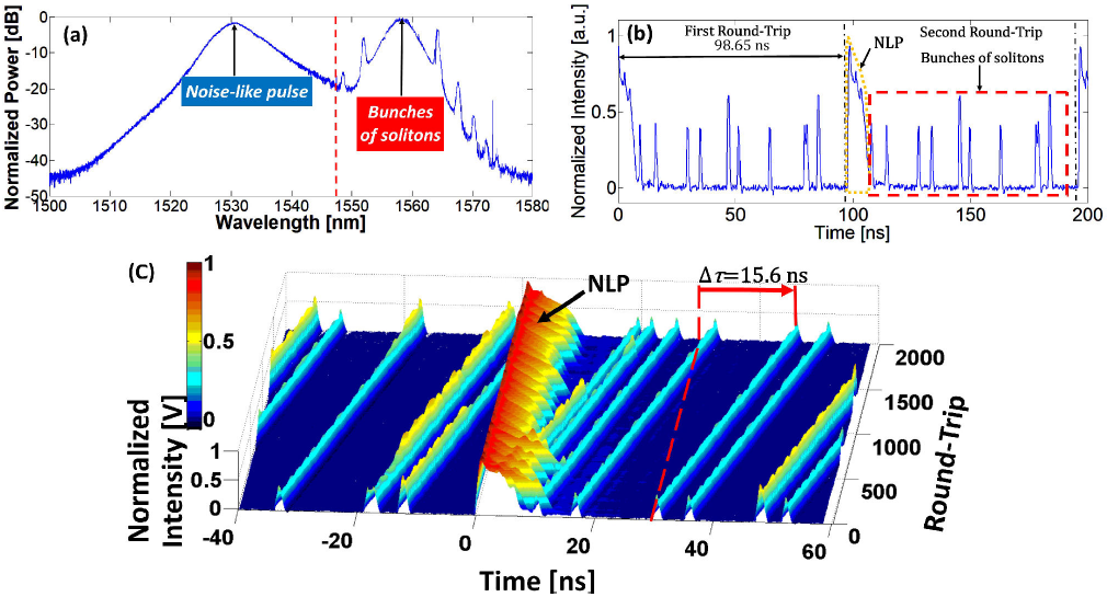
Figure 9. Regime of NLP and bunches of solitons. a) Optical spectrum. b) Temporal profile along two consecutive round-trips. c) 3D mapping of the temporal profile evolution along 2000 round-trips, the temporal walk-off is indicated (15.6 ns in 2000 round-trips)
Since the pulses correspond to different spectral components, the NLP and the bunches of
solitons have different velocities with respect to each other. Besides, the
anomalous dispersion in the cavity ensures that the bunches of solitons
(longer-wavelength component, 1558 nm) are delayed with respect to the NLP
(shorter wavelength component, 1531 nm). Fig.
9c shows the 3D mapping of the pulses temporal profile for this
regime, which is similar to the case illustrated in Fig. 7b; in this case the NLP presents a fixed position over
2000 round-trips and the bunches of solitons have a temporal walk-off (to the
right) of 15.6 ns along 2000 round-trips (7.8 ps per round-trip), this
experimental displacement is consistent with the theoretical temporal walk-off
per round-trip of Eq. 16 (considering the total dispersion of the cavity
D
T
= 0.285 ps/nm and the spacing between the two spectral components
5. Final comments
In this work, the basic elements in a PML-FRL were studied, in particular the SA mechanism achieved through NPR, and the use of linear polarizer was analyzed theoretically. It is important to note that in an experimental setup of PML-FRL, a uniform twist applied to the optical fiber introduces circular birefringence that rotates the polarization ellipse along propagation but does not alter its ellipticity, which ensures that NPR is uniform along the fiber, similarly to the theoretical study in Sec. 3 of the NPR effect in an isotropic fiber.
In general, the 3D mapping measurement provides deep information about the pulse dynamics, including their interactions and the behavior of the temporal envelope. This work focused in the study of the 3D mapping measurement of a pulse conglomerate coexisting with a single pulse that correspond to different wavelength components in anomalous or normal dispersion regimes; the simulated behavior is contrasted with experimental results in which pulses associated with two different wavelength components coexist. The behavior in time domain tends to present one pulse or a group of pulses with fixed temporal position over successive round-trips, whereas the pulses associated with the other spectral component presents a temporal walk-off to the left or right. Besides, when only one spectral component exist, the 3D mapping measurement only shows pulses with fixed position over successive round-trips, as it can be observed for example in 34; or in this case all pulses present a fixed temporal walk-off, as shown in 45.

