


 nova página do texto(beta)
 Inglês (pdf)
 Artigo em XML
 Referências do artigo
 Enviar este artigo por email
 Citado por SciELO
  Similares em
SciELO
Similares em
SciELO 
 Permalink
PACS: 01; 07; 47
1. Introducction
Flow of liquids or gases is commonly present in heating, chilling and hydraulic distribution network systems, where a typical array includes pipes of several diameters, valves, different types of fittings and pumps, where these devices are used to pressurize flow, control flux and change flow’s direction. Even though the theory of fluid flow is reasonably understood, theoretical solutions are found only for some simple cases, such as laminar flow completely developed in a circular pipe. Therefore, theory should be backed up with experimental results and empiric relations for many of fluid flow problems, instead of having exclusively analytical solutions. On the other hand, it is important to observe fluid behaviour at different velocities to clearly comprehend fluid phenomena, which is characterized by the dimensionless Reynolds number.
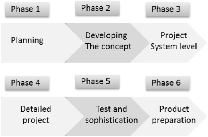
Development of the system proposed in this work was carried out following the Product design and development (PDD) methodology depicted in Fig. 1.
2. Equipment design concept development and detail
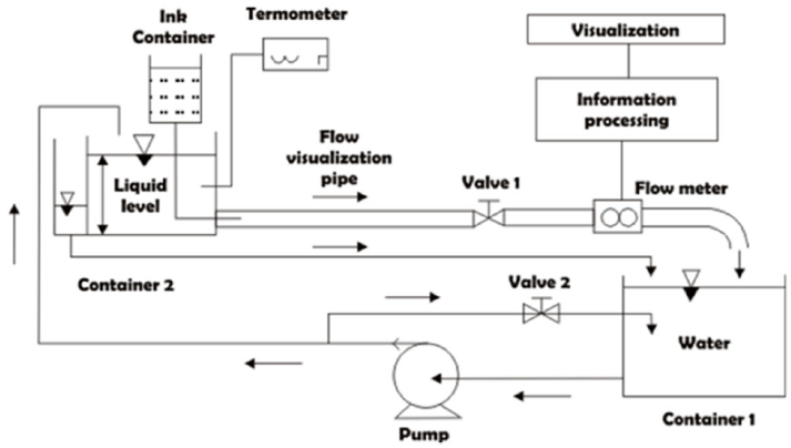
Design process consists on converting needs and requirements into useful products. Problem is looked into and project’s scope is defined. In this stage, the factors discussed in the following sections were taken into account to come up with the proposed equipment shown in Fig. 2.
2.1. Water containers
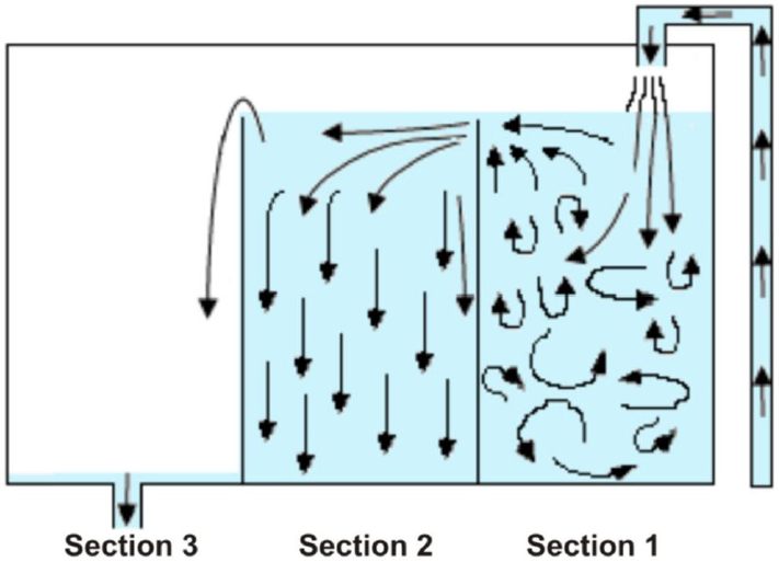
The prototype includes two water containers or tanks, the first container is connected to a pump which provides it with water. The second container is divided into three sections. The first section is filled up with water coming from the first container so that turbulence caused by water dropping does not affect the other sections.
A thermometer is connected in this section to collect data for density and viscosity calculations. When water fills the first sectioncompletely and reaches the high of a wall that separates sections, it starts to drain to the next section without causing turbulence since it flows smoothly over the division. The second section provides the necessary fluid for the experiment; when fluid has constant height, experiment is started by opening valve 1 to permit the liquid to flow across a visualization pipe and through a flow meter to know flow velocity. In this section flow behaviour is observed by injecting ink in order to color stream lines. The fluid in the second section eventually will fill and drain to the third section and will then return to the first container to start the cycle all over again, Fig. 3.
2.2. Diameter selection of visualization pipe
Piping dimensions were calculated based in the following equipment and their characteristics: water pump, flow meter and material of visualization pipes, either glass or acrylic.
2.3. Water pump selection
According to the usage of this device, the pump selected is of submersible type, lightweight, easy installation, silent and with a capacity of 2.92 × 10⁻⁴ m3 s-1 (Fig. 4a).
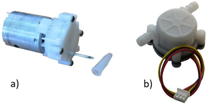
2.4. Flow meter
Hall flow meter type was selected (Fig. 4b), which consists in a turbine that spins when fluid crosses it and produces a series of pulses that are proportional to the flux passing through a sensor. Commercially, flow meter with nominal diameter 12.7 mm is able to measure in the range 8.33 × 10⁻⁶ to 5×10⁻⁴ m3 s-1, and the 25.4 mm flow meter can deal with 3.33 × 10⁻⁵ up to 1.67 × 10⁻³ m3 s-1.
2.5. Pipe selection
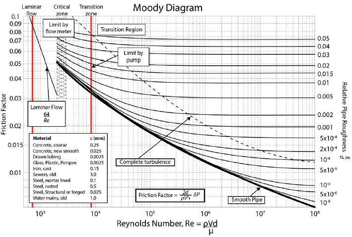
Commercially available transparent pipes, made either of glass or acrylic and able to connect adequately to flow meters have 12.7, 19.05 and 25.4 mm in diameter. Consequently, an analysis was carried out to determine the interval of Re numbers that might be visualized and measured for the different combinations of diameters and flux sensors, based on the minimum fluxes that sensors were able to detect and the maximum volume displaced by the pump, taking into account material’s roughness 14.
Combination of 19.05 mm pipe and 12.7 mm flow meter gave the largest interval of Reynolds numbers to be measured in this equipment (Fig. 5). Such range includes Re numbers from 800 up to 28000.
Another important aspect in the design of this system is the length of the visualization pipe. Such length is determined by taking into account the inlet length Le, which is the region where the flux has not yet developed completely.
Velocity profile in the region where flow is totally developed has a parabolic shape in laminar flow, and it is flatter in turbulent regime due to vortex movement and vigorous flow mix in radial direction (Fig. 6).

In laminar regime, hydrodynamic inlet length Le lam is approximated with the following expression 1,2,3,4:
where Re is the Reynolds number and d is the pipe diameter. In turbulent regime, the intense mixture during random fluctuations usually hides molecular diffusion effects. Inlet length for turbulent flow Le turb is approximated with 1,2,3,4:
Figure 7 shows theoretical inlet lengths (in mm) needed to develop completely the velocity profiles that correspond to laminar Reynolds numbers (L Reynolds = L ent ) for different design conditions; visualization lengths are also shown for each inlet lenght. For turbulent flows, it was observed that profiles are closer to each other than in the case of laminar flow.
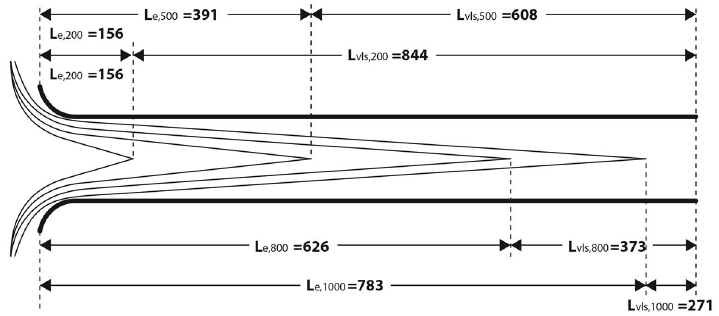
A 1000 mm pipe was selected from these results. These measurements were corroborated with a finite element analysis 5,6,7,8,9 ran in ANSYS® for different Reynolds numbers: 800, 1000, 4000 and 10000.
Velocities for each Reynolds numbers (inlet condition, left hand arrows), atmospheric pressure (outlet condition, right hand arrows) and walls (pipe) dimensions were taken as boundary parameters for the simulation.
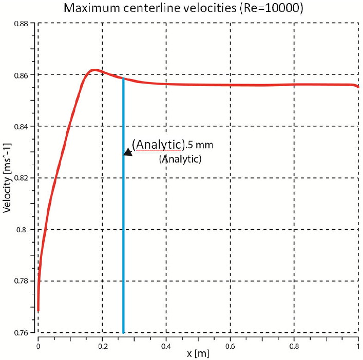
Results from ANSYS® Fluent for Reynolds number of 10000 are shown in Fig. 8 as an example. Velocity change throughout centerline of the pipe can be seen in red; when fluid reaches the inlet length, velocity becomes constant. Both numerical and analytical results are presented in the figure. After velocity profile surpassed the inlet length, it remains constant for the rest of the pipe.
2.6. Calculation of heights
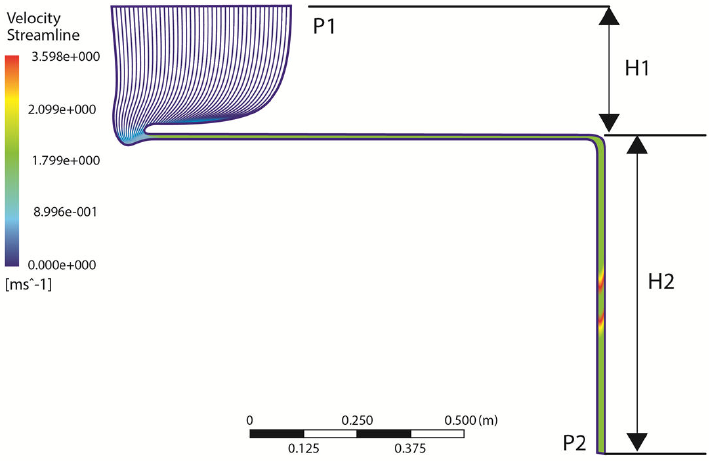
Energy conservation equation is used to know the heights between any points 1 and 2 1,2,3, necessary to know velocities that the system will be able to reach (Fig. 10).
Where P is pressure, V is speed, H is elevation from a reference,
Where Ki are energy losses due to system’s features: Kcg denotes gradual contractions, Kf indicates friction, Kv relates to valve, Keb and Kcb are losses in flow sensor and Kc means 90° bends.
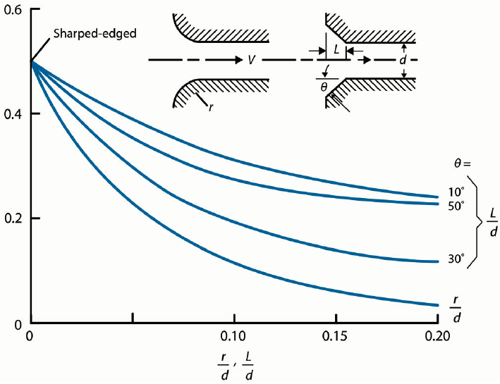
In the case of Kcg , a relation r = d > 1 was proposed for gradual connections in the equipment, where r is the radio of the fillet and d the diameter of the pipe, Fig. 9. Friction losses are calculated for flow in turbulent state since it is not possible to know valve’s opening size 10,11,12,13 and the maximum height of equipment corresponds to the largest Reynolds number, i.e., in turbulent regime.
A friction factor value
As the Reynolds number grows, height H1+H2 also increases because more potential energy is needed to accelerate the fluid. Table I shows this behavior.
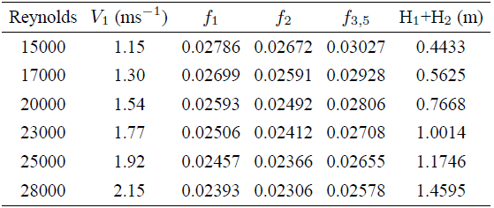
From an optimization point of view, a height of 1.0 m is chosen for this testing equipment, expecting to obtain a maximum Reynolds number of 23000 and a visualization velocity in the pipe of 1.77 m s-1. Once system’s configuration is set, simulations are carried out in Ansys® Workbench (Fig. 10). Simulation results were used to build a system’s prototype. Boundary conditions are: atmospheric pressure at inlet and outlet points, pipe’s wall, and gravitational acceleration equals 9.81 m s-2 in vertical direction. Simulation’s results give the velocities at different sections in the system.
Figure 10 shows flow simulation through the system. Results highlight that velocity in the visualization pipe is close to 1.79 m s-1 which is slightly above the analytical result of 1.77 m s-1.
Velocities V2 through V5 in each
section of piping are calculated using the equation of continuity, for example,
for Sec. 2,
Comparison of these values with simulations in Fig. 10, demonstrates that both values match for every section.
3. Equipment construction and testing
Scheme in Fig. 11 shows the various equipment’s subsystems. Construction of equipment required the use of additive manufacturing (3D printing), Computer Aided Manufacturing (CAM) and conventional cutting and assembly processes.
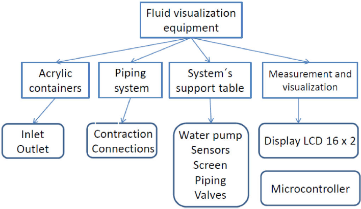
Figure 12 displays final design after construction of parts and assembly 15,16,17,18,19.
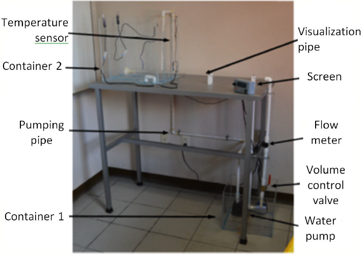
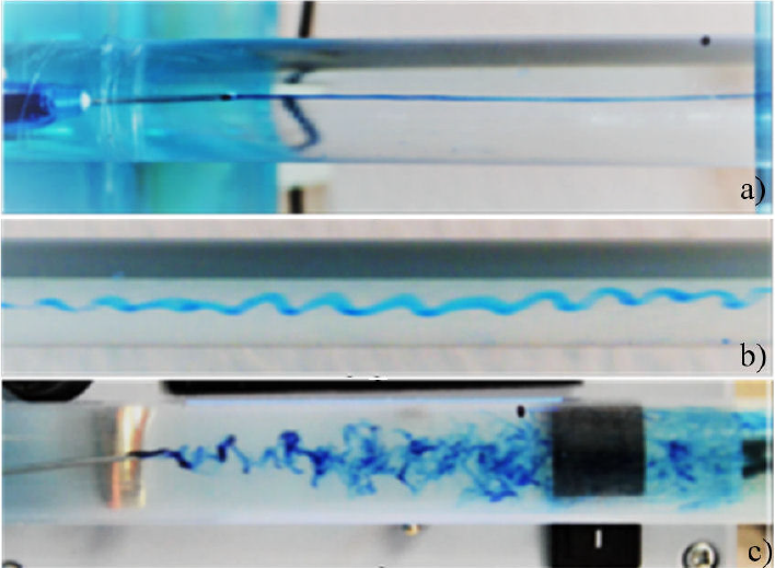
Figure 13 exhibits how the equipment is used to visualize fluid at three types of flow regimes by injecting ink to the fluid. The equipment has maximum measures of 0.60 m wide by 1.20 m long and 1.20 m high.
Several testing runs were carried out for different Re; in order to know about several fluid’s parameters at any time, a display was implemented to measure them. Through this device, the user of the equipment is able to read fluid’s velocity, temperature and Re right from the screen, as depicted in Fig. 14. This is a core characteristic of the equipment since other equipments do not have such capability and the user can not know about fluid’s characteristics.
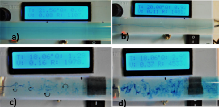
Figure 14. a) laminar flow, Re = 1107, b) transient Re = 1481, c) turbulent Re = 1978, and d) turbulent Re = 4533.
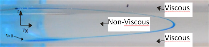
On the other hand, velocity distribution in pipe’s cross-sectional area can be visualized. The “no-sliding” effect can be observed so that ink particles next to pipe’s wall adhere to it and stay at zero velocity, whereas velocity is maximum at the center of pipe, having a parabolic profile as shown in Fig. 15. It is also possible to see the development of the boundary layer in this figure; viscous and non-viscous zones are clearly distinguished, meaning that as flow increases, viscous layers unite and finally all the flow becomes viscous.
4. Conclusions
It was observed experimentally that working with fluids requires precision and close control of conditions in order to have coherent results, especially at high speeds (1000 < Re < 10000). At low speeds (Re < 1000), flow is laminar despite any disturbance may exist. This equipment was designed to work with Re numbers up to 23000, however, it was evident from testing runs that it is not necessary to use high Re numbers from a didactic standpoint, which is the main goal of this equipment; it permits observation of fluids behavior as well as reproduction of Osborne Reynolds’ experiments carried out circa 1883 20.
Flow velocity measurements has an error of ± 10% associated with flow meter. Microcontroller’s working frequency is configured at 16 MHz to reduce error and to sense with enough speed since maximum frequency is 75 Hz. In the final characterization of the equipment, it was possible to measure Re numbers between 800 and 23000 as expected.
This design offers a novel way to visualize different flow types of incompressible fluids in piping since it allows the user to make readings directly from apparatus’ screen. Temperature, velocity and Re are the parameters that can be taken. With this capability, users can verify theoretical calculations against data taken with the display; additionaly they can easily realize as Re grows, fluid behavior changes from laminar to turbulent regime.

