


 nova página do texto(beta)
 Inglês (pdf)
 Artigo em XML
 Referências do artigo
 Enviar este artigo por email
 Citado por SciELO
  Similares em
SciELO
Similares em
SciELO 
 Permalink
PACS: 43.75.De; 43.75.Yy; 43.75.Cd
1. Introduction
Often, the sciences and engineering knowledge is not easy for transmitting with only theory. Teaching-learning process immerse in a model based in competences can use virtual and experimental tools in order to facilitate this process. For this reason, the Computer Aided Instruction (CAI), as pedagogical tool, has complemented the teaching-learning process for improve the understood of the students, particularly in science and engineering education 1,2, and in special about vibratory analysis.
Experiments using spectrum analyzers, as well as mathematical software and numerical simulations have been used for teaching acoustics and vibrations, for both textbooks and educational papers. Besides, advances in computers have allowed that several equivalent tools can be available for students to facilitate these kinds of activities 3.
Unfortunately, the cost of licensed commercial software and the incompatibility between operating systems currently used (Windows, Mac OSX, Linux, Android, iO), as well as the lack of equipment for vibration measurements; restrict the implementation of several developments available for teachers. Avoiding all these restrictions is desirable for teaching vibrations, so the aim of the present paper was applying free tools for experimental, theoretical, and numerical procedures for this purpose. Such a confluence is hard to find, at least for the authors, in other papers about teaching vibrations.
For example, the use of a spectrum analyzer to impart a course of acoustics has been successfully reported previously in 4. However, the type of analyzer and microphones reported in such work implies a substantial investment in equipment; also, the use of this kind of instrumentation to measure vibrations requires background in experimental mechanics that, while it is available in literature e.g.5, usually this knowledge is not vastly studied in courses of mechanical vibrations. Alternatives as LabVIEW have proved to be useful in teaching modal analysis 6, but the cost of the licensed software is high. It seems feasible substituting some conventional devices as oscilloscopes, spectrum analyzers, and interfaces, through computers or even smartphones capitalizing on the increasing familiarity of students to use these new devices; because according to recent studies 7, students who own smartphones are largely unaware of their potential to support learning, but they are interested in and open to the potential as they become familiar with the possibilities for a range of purposes.
On the other hand, in recent versions of textbooks about vibrations, Matlab is another expensive software which often appears to obtain graphics and calculus of suggested activities. In some cases the proposed exercises using Matlab even require special toolboxes, e.g. 8,9. However, in other cases the activities only are written with basic functions of Matlab, e.g.10, and it could well use free software; or even some recent textbooks and papers are being written including examples which use free software exclusively, e.g.11,12.
For the case of teaching mechanical vibrations, using simulations usually involves expensive software. Such is the case for the textbook of 9 which in addition to using Matlab, ANSYS is needed to apply the finite element method (FEM). FEM is a powerful numerical technique employed to analyze dynamical systems and a good introduction to this topic is found in Ref. 13. Some interesting alternatives of using FEM as teaching tool are available. For example, 14 simulated mode shapes of a plate through software developed by the first author of such work, Visual FEA, which is software based on FEM; however, its free version is limited in time and number of nodes, and while VisualFEA works under Windows and OSX, Linux is not supported. Both the lack of supporting several operating systems and using trial versions of software have resulted in complications for the authors of the present paper, implementing procedures with such limitations in previous works of the authors 15,16.
In view of all these, the activities for simulation and experimentation for this work were designed with the aim that students interested in introductory studies of vibrations (even without strong background in physics) acquire the competence know-know and know-do. For this task, free computational tools, with complete and cross-platform versions without restrictions, were applied to analyze real vibratory systems through the confluence of three different procedures: numerical procedures (FEM), theoretical developments, and experiments. Therefore, the student acquires the knowledge and bears out with simulations and experiments, reaching the goal competences.
While this report is finished with some practical examples, the main procedures were focused to free vibrations of beams for two important reasons: 1. Theoretical developments and simulations of beams are simple but they allow explaining the same topics occurred on much more complicated structures. 2. The facility for all the students to perform their own experiment, because finding one beam per each student is not a hard task.
2. Modal behavior of beams
From an analysis in frequency domain of a structure, obtaining complete information about its dynamical behavior is feasible if the structure is excited by an impulse as input and measuring the output response. For practical purposes, a very short input compared with the time constants of the system can be considered as an impulse 8.
The lowest resonant frequency of a free beam can be extracted from a frequency response function, as the impulse response. Following the peak-amplitude method 5, it is known that from detecting the first individual peak of this impulse response, the frequency of maximum response taken will be the natural frequency of the first free mode.
The description of the deflection shape of the beam at this first natural frequency, i.e. its mode shape, is easy to find in literature 10. In the present work the first free mode of beams was analyzed, whose transversal vibration y for any x point of an unitary beam can be approximated entering the code:
at any math software. For such task, the use of free software working under the same commands of Matlab is suggested. Octave 17 was used here because it is compatible even with Android smartphones. Also Scilab 18 can be used with the same commands, and while it does not have mobile version or it does not try to clone Matlab (as Octave), Scilab installation is easier under Windows and OSx, for a good introduction see 11. Octave and Scilab are open source. It is recommended asking that students use any free application with these features instead of the calculator of their smartphones, with the aim to familiarize them for solving the exercises of Matlab included in other textbooks. For example, several proposed exercises at 10 can be successfully executed directly in a Scilab environment. Obtaining the graph for the first free mode shape of a beam, simply by using plot(x,y), was the starting point of the activities performed by the students.
2.1. Slender beams
Two beams of solid material were used for the experiments, whose length is greater than width, and much greater than its thickness. One of these beams was a one-meter aluminum beam, the other was a wood beam (spruce) of 200 × 20 × 3 mm. Students performed the experiment individually, using their own bar, once that the teacher showed how it must be done.
2.2. Boundary conditions and applied forces
Strictly speaking, reaching free boundary conditions during experiments is impossible; even so, some practical tips are useful to show success. A technique trying to reach free boundary conditions implies holding or supporting softly the experimental beam over any of the nodal lines of a mode shape to being analyzed; in this way, the beam will tend to vibrate freely for this mode shape. On the other hand, the best places to drive a free structure are the edges, because it is expected that the edges will exhibit maximum amplitudes of vibration.
2.3. Impulse response
The aluminum beam was used for naked-eye detection of the first mode shape of a free beam, as well as to explain the concept of nodal lines. For this purpose, the beam was held with two fingers while it was tapped using the fingertip of the other hand. Once the beam was vibrating, the beam was touched over other nodal line to show that such additional conditions should not modify the analyzed vibrational state.
After, an impulse response was obtained from the wood beam as demonstration of the experiment performed by the students. The driving force was applied to the wood beam impinging it using the nails. The radiated sound by knocking the wood beam was captured as output signal, using microphone through free spectrum analyzers. The software installed for this task were SpecScope 19 under Android and AudioXplorer 20 under Mac OS x ver. 10.9.5; in both cases, the sound was recorded using the integrated microphone in the devices. Under Windows, Visual Analyzer 21 was installed and a generic microphone plugged to the multimedia port was used. It is worth mentioning that both AudioXplorer and Visual Analyzer also offer oscilloscope and signal generator which can be very useful.
3. Finite element simulation
A modal analysis of a wood beam model was simulated through FEM. Finite element (FE) simulation is a systematic and modular numerical technique. Results from such calculations lets us analyze precisely the vibration of a structure by the movement of nodes, connected by lines of an element grid, on the discretized model 10. The basis for FE implementations imply strong theoretical developments (e.g. see 13), but using dedicated software greatly facilitates the steps to perform a FE simulation; were the user-program interaction is carried out by a generally intuitive interface. FreeCAD 22 was used to create the geometric model, while Aurora Z88 23 was used for the FE analysis. Both programs are freely available and cross-platform; specifically, they were succesfully installed in Windows 7 and OS X ver. 10.9.5 (Linux versions are also available but they were not tested).
3.1. Geometry definition
The first step for any FE analysis is to build the geometric model. The sequence of such process is described as followed. Once the program FreeCAD is open, wait until all the interface tools are completely loaded. Then, start a sketch by pressing the button: Create Sketch, as indicated in Fig. 1A. Subsequently, define the type of work to be performed by pressing the tab: Part Design (Fig. 1B), in order to assign the design task to the sketch.

Afterward, a dialog box appears asking to define the Cartesian coordinates on the work plane, according to the reference axes of a cube. Conventionally, the Cartesian plane used as a first instance is the X-Y plane. However, the Cartesian plane selection is arbitrary. The next step is to proceed to draw a rectangle in the Cartesian plane with arbitrary dimensions, pressing the button for such geometry (Fig. 1C).
In order to define the scale of the rectangular geometry according to experimental data, the length and width of the rectangle are dimensioned with 200 mm and 20 mm, respectively, using the dimensioning tool (Fig. 1D). Conclude the process of the bidimensional geometric definition in the sketch, pressing the button: Close (Fig. 1E).
In the last step, the three dimensional geometric definition is carried out with the plate thickness. Then, the rectangle is extruded 3 mm at the Z direction by using the extrusion parameters tab, which is activated pressing the button: extrusion (Fig. 1F).
Importantly, as discussed in the next topic, the geometry must have appropriate tolerances and continuities for a correct finite element meshing. In addition, changing some endings helps to simplify processes of geometric operations, which can be considered as negligible for the analysis, such as rounding of edges, chamfers, etc.
Finally, the geometry is exported displaying the tab File Export as, and selecting export as a file with the extension *.stp.
3.2. FE model
Regarding the simulation, AuroraZ88 program allows importing geometries created in computer-aided design, CAD, in order to perform calculations through the FE. The simulation process consists of three steps: preprocessing, calculations, and post processing 24.
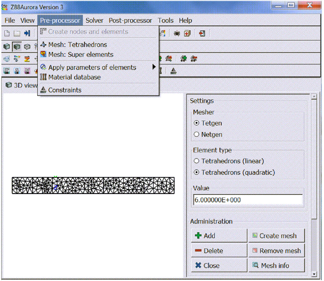
The first step of preprocessing is to define the characteristics of the simulation type, as well as the respective material properties, to be associated with the model. For the case of AuroraZ88 program, a new job is opened, where an empty folder is selected to save the corresponding files. The geometry is imported by displaying the tab Import File option and select the file with *.stp extension, previously generated in the FreeCAD program. Then, the meshing type is defined in the Pre-processor tab, the open Mesh option is selected and proceeds to choose Tetrahedric elements. In order to specify the characteristics of the mesh, again the Pre-processor tab, opens the mesh generation option TetGen and select quadratic as the element type. In the same way, a value of 6 is assigned, which is related to the size of the elements to be created, see Fig. 2.
The material properties are defined through the Pre-processor tab, where a Material database available is selected. The unit system can be modified by the user, see Fig. 3. In order to have compatibility with the units system of materials already included in AuroraZ88, viz. mm/t/N units (see its user-guide); i.e. millimeter/ton/newton. It proceeds to define the density measured experimentally, 4.8e-10 t/mm3. Later on, enter a Young’s modulus of 21200 N/mm2, and a Poisson’s ratio = 0.40, which values were estimated from the expected range for the spruce 25.

Subsequently, the simulation type is defined in the calculation step. In the present case, it is required to perform a modal simulation, which is assigned to the calculation process using the upper left tab Free vibration. Select the Solve option, use Lanczos and Open in Solver and Solver parameters options, respectively, and Start is selected.
It is responsibility of the user to ensure that the mesh obtained provides consistent results. One of the criteria to consider is about the size of the mesh elements, which should decrease until no significant changes in the results are obtained, in relation to acceptable experimental values.
Finally, at the post-processor step, display the menu on the right side of the program interface, and select visualize the solution of the eigenvalues of the second vibration mode. Specify the values of displacement to display in the Z direction and the beam geometry without deformation, in range of red-blue and black lines, respectively.
It is noteworthy that these procedures for FEM implementation were calibrated by means of an engineering student, into the framework of the Delfin-CONACYT program 26. The aim of his project was to perform the FE model and simulation, without help from the advisor, in order to adjust each complication as reported by the student to improve the final procedure instructions.
4. Results and discussions
4.1. First mode evaluation
The contour of the beam deflection, regarding the first free mode, is shown in Fig. 4. Through the Octave software for Android system, the contour of the deflected beam was built running the two-line code in Sec. 2. Also, the undeflected beam contour was included. Scanning the graph of Fig. 4 (right) allowed to detect the nodal points, which are located at a distance of 0.22L from the beam ends. In addition, the antinodes were located at the beam ends. Given such boundary conditions, the aluminum beam was excited to vibrate at its first free mode, as can be seen in Fig. 4 (left).
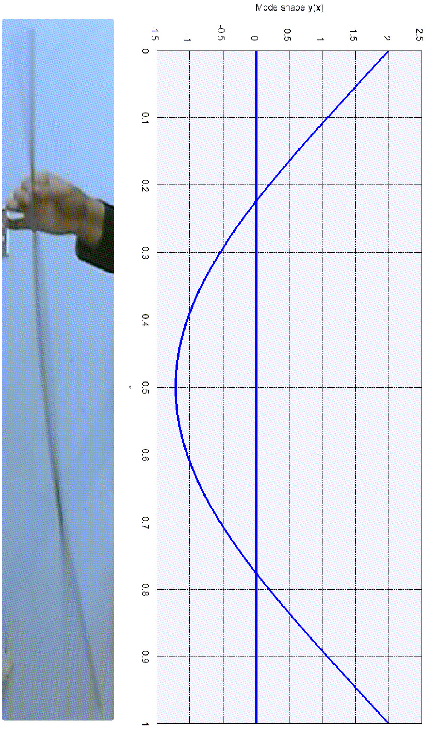
Figure 4. Experimental and theoretical result at the first vibration mode of the free aluminum beam.
In the present case, the maximum displacement was in centimeters order, and the natural vibration mode had a considerably low frequency; then no additional instrumentation than the reported was necessary to measure the experimental data. Some calculations with damping present, between the beam and the air, do not show differences when compared with damping-free case, thus the last choice was used. However, as additional consideration, in order to quantify part of the dissipated energy through the air, a microphone should be required to record the sound produced at such frequency level. The magnitudes and scales where damping effects had relevance in calculations results will be considered for future studies.
4.2. Resonance frequency detection
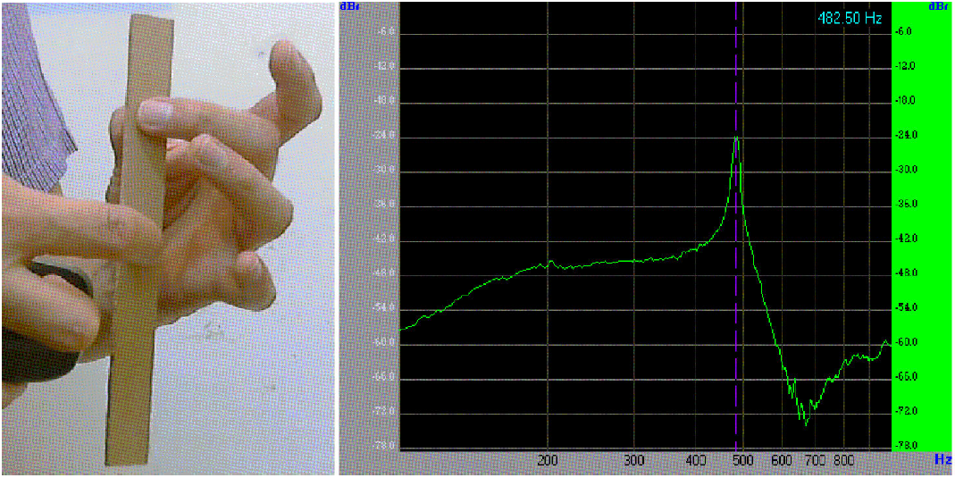
In the same way, similar boundaries conditions as for the aluminum beam were assigned to a wood beam. For instance, a subjection nodal point was located at a 0.22L distance from the beam end as shows Fig. 5; while the opposite free beam end was defined as the excitation point. For the case of the wood beam, the first vibration mode was no longer visible to the naked eye, or far higher modes. However, in this case the sound was perceived to the human ear, where the continuous signal of sound, without a sudden stop, supports that an adequate behavior was obtained. In fact, the defined conditions allowed performing correctly an impulse response, c.f. Bode plots in [8], in order to create an enough deformation magnitude of the wood beam. As a result, the first resonance frequency was clearly detected at 482.5 Hz, which corresponded to the first free vibration mode, according to the deformation mode of the beam shape. Therefore, the aim of the present work was to obtain a spectrum, with no more specially designed device for this purpose, as it was few years ago 27, since you can simply emulate its operation, following these procedures.
4.3. FE simulation results
The patterns of the wood beam discretized by FE modeling, without bending and with the deflection at the first free vibration mode, are shown in Fig. 6. The comparison of the total displacements values calculated from the modal simulation, against the experimental data in Fig. 6, showed a very well matching. Regarding the resonant frequency, the first vibration mode was calculated at a frequency of 482.8 Hz. Such calculation was obtained when the estimated values of 400 kg/m3 and 21.2 GPa for density and Young’s modulus, respectively, were used in the FE simulation. Accordingly, such Young’s modulus value is very close to the expected range data from 10 to 20 GPa for spruce wood 25. Thus, the combined analysis of the dynamic response of a beam with the iteration of the elastic property defined into the FE model, can be used as an approximation process to find the correct value. Consequently, several FE simulations should be run until the computed results converge adequately with the experimental measurements, in order to characterize with a high-accuracy the Young’s modulus of the tested material.

It is important to take into account in the interpretation of the results that the simulation must have effects due to the ideal conditions and optimizations, defined at the construction model step. Furthermore, the FE simulation could carry implicit errors from the solution method. Then, the user should keep in mind how much the results change due to each parameter that constitute the model and simulation. Thus, the user should have the capability to define properly each assumption and simplification made during these processes, in order to provide a convincing FE analysis.
5. Reception by students
Once these free tools were used by the students, they themselves developed spin-off projects at this respect. Some cases were here included as examples. By way of introduction, related opinions of different groups of students of engineering at Universidad Anáhuac Campus Querétaro were collected, once these tools were implemented in their classroom.
Some details of the usefulness of procedures here described were taken from students of acoustics of the violin, a classic topic where Mexican research begins to emerge (e.g.28). Finally, another example was about final projects of a course of Introduction to FEM, imparted on a master’s degree program of CIMAV-Monterrey.
5.1. Feedback from engineering students
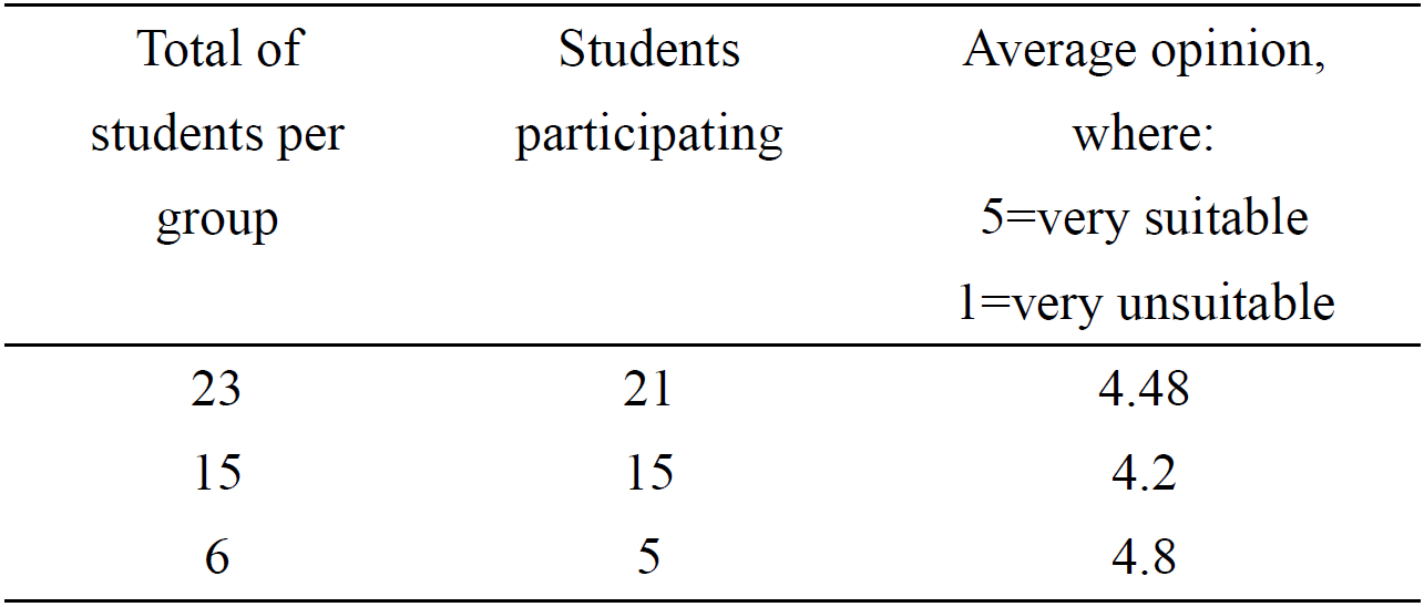
The choice and usefulness of the computational tools here described were evaluated by three different groups after being implemented in their classroom. Their opinions were summarized on Table I, showing a positive reception for the three students groups, since the obtained evaluation exceeded 4/5 for all the cases. In addition, one student chosen randomly commented that the explained concepts in classroom were complicated, but using these computational tools made it easier.
5.2. Students of violin making
All the current students of Escuela de Laudería said that before the Acoustics course they did not know anything about the kind of software used in the present work; however, 70% of them still use it after the course. Spectrum analyzers have been the most popular tool, largely due to feasibility of being installed on mobile devices. Also, violin making students have applied the procedures here described, in order to obtain the Young’s modulus of wood samples used in their workshops.
Several students employ some of the software described in this paper to develop thesis; for example 29. In this cited thesis, violin top plates, i.e. the plates with f-holes, were analyzed because useful information for violin making can be be extracted from the resonance frequency of them. Fig. 7 shows both modes and the experimental set-up developed by the student for this purpose.

Figure 7. Chladni patterns of the second and fifth free modes of a violin top plate, and experiment to measure the resonant frequencies of a free violin top plate; as it was reported in a thesis of violin making 29.
5.3. FE master degree course
On the projects of this course, the construction and deformation of two structures of aluminum were made: a can and a bicycle frame. Both structures were subjected to a combination of compression and tensions stresses, within the elastic regime, and the total-displacements caused were analyzed. The corresponding FreeCAD models and their FEM results calculated in AuroraZ88 are shown in Fig. 8.

Some difficulties and conclusions highlighted by students when they had in carrying out the work were collected, viz.:
One of the main technical difficulties when starting to work with both programs had been when trying to save, import or open files with FreeCad or AuroraZ88. Then, it has been observed that both programs have difficulty regarding to their management files algorithm, for example when files have been saved into subfolders. As a result, the given solution was to create folders directly on the desktop or in the main directory.
When a meshing model process is carried out for a first time, it is not so aware that increases in the amount of elements that constitute the mesh, normally increase exponentially the computation time for the FEM solution. Therefore, once such effect is faced; efforts to solve the model with a coarse mesh must be taken. Thus, the necessity to develop meshing criteria takes place, such as the exposed in class of decrease the amount of elements in such parts where it is expected the simulations results are not so relevant.
The simplification of simulations becomes important when the computing capacity begins to be limited, particularly for the cases of three-dimensional models. So once the user begins to have difficulties in pre-processing or post-processing data steps, the three-dimensional models begin to be proposed as simpler models. For example, in some three-dimensional simulations it was necessary to develop simplifications, either through mirrored symmetry planes, axisymmetric axes, or models that can be analyzed with an extruded two-dimensional solution. It was concluded that before begin to build three-dimensional models, one must consider firstly the possibility of its representation by two-dimensional models, which normally applies to cases where geometries as well as constrain conditions are symmetrical.
6. Conclusions
The support provided by free cross-platform software on understood vibrational concepts was practically well received among students. The analytical, experimental and numerical activities simultaneously performed, motivate students to deepen in the usage of software-tools in order to simulate dynamical behaviors, and experimental tools as spectrum analyzers are still being used in violin making workshops of graduated students.
Concerning to FEM simulations, even though a model has been built with a representation apparently as appropriate as possible to a real problem, and additionally has been carried out solutions of possible alternative behaviors of the system; the results of the simulations differ from the experimental results. Until then, the user begins to understand that real system it is may be affected by additional external excitations from the environment, which apparently were not so significant at the time of carrying out a preliminary analysis. Such considerations begin to have an important role when it is done the feedback through a more meticulous study, trying to simulate a phenomenon as close as possible to the reality.
For the case of FreeCAD, it is interesting that the built geometries can be exported with compatible extensions for a great variety of FEM simulation programs, so it would be interesting to solve the same problem using others FEM programs and try to understand their differences. Such conclusion could be used in order to consider an additional feedback to advantages and limitations analysis that each program has, as well as the scope of its respective results validity, considering how far are their solutions from the real problem.
It is very helpful to have a well-established procedure as used in classes (which agrees with the described in the present work), since although it is practical to watch tutorials videos or read verification manuals when learning how to use some tools for both programs, many times such tutorials are not easily available, not well described or developed, or do not manage the respective exercise with a well-established procedure. In addition, sometimes such sources do not clarify the consequences if the steps order or some assignments considered are modified.
The fact students have easier access to internet connection, smart devices, and free software; enables them to use the advantages explained in this work:
The usage of third-parties computers, which requires administrative activities, is not necessary because all the students will work with his/her equipment regardless of operative system installed.
Software is installed by students on their own devices, without help of teacher or technical staff.
Exchange of files through removal drives does not exist, because software is available online.
According to the established goals, practically any computer or mobile device is enough in order to perform the activities shown in this work.
The students acquire the knowledge and do experiments and simulations, so the know-know and know-do competences were achieved.
Therefore, teaching the vibratory behavior to students can be actually complicated, because this topic involves difficult concepts of picturing. However, computational tools help the explanation by teacher in the classroom. This latest was possible because students can use their computers, or even smartphones with more processing capabilities than their teachers used in order to learn.

