1. Introduction

In 1662 Robert Boyle made several experiments in order to demonstrate that the pressure of a gas and his volume were in reciprocal proportion ^1,2, arriving to what today is called Boyle’s law:

Looking at Eq. (1) the following question can be made: Which is the value of this constant?

This is a question that can be made to the students of a general course of physics for learning the laws of gases. The answer can be obtained from an experimental point of view; to do that, several proposals can be found in the literature that describe Boyle’s law apparatus for a student laboratory and that explain how to use the experimental data to deduce the relationship between volume and pressure of a gas ^3,4,5. But not always experimentation can be carried out. In this case, it is proposed to recover the historical data of the experiments that led or contributed to the laws that nowadays are studied, to obtain valuable information from them. Such data was obtained in many cases with a lot of effort and great precision ⁶. In this article, an answer to the previous question will be proposed through the analysis of the original data obtained by Boyle in the experiment that he made in 1662.

2. Boyle’s experiment

A very detailed description of the historical experiment that led to Boyle’s law can be found in the Part II, chapter V of the Boyle’s book published in 1662 ⁶, and also in the literature ^1,2.

Boyle used a glass tube bended in an U shape having one short leg hermetically closed in its top part and containing a fixed quantity of air in it. He poured mercury into the long leg to compress the air in the short leg. Both legs had scales in inches to measure the height of the cylinder of air in the short leg and the height of the cylinder of mercury in the long leg that was compressing the air.

In the description that Boyle made of the experiment, two parts can be distinguished; in the first part is described the way employed in obtaining an equilibrium state in which there was no height of mercurial cylinder compressing the air, but only the atmospheric pressure. In the second part is described the way of pouring mercury into the longer tube and the way of taking experimental data, as Boyle explains in his book (6):

Then Quicksilver being poured in to fill up the bended part of the Glass, that the surface of it in either leg might rest in the same Horizontal line, as we lately taught, there was more and more Quicksilver poured into the longer Tube; and notice being watchfully taken how far the mercury was raisen in that longer Tube, when it appeared to have ascended to any of the divisions in the shorter Tube. Thus successively made, and as they were made set down, afforded us the ensuing Table.

The data of original Boyle’s experiment is presented in Table I.

Table I. Original Boyle’s experiment data. 

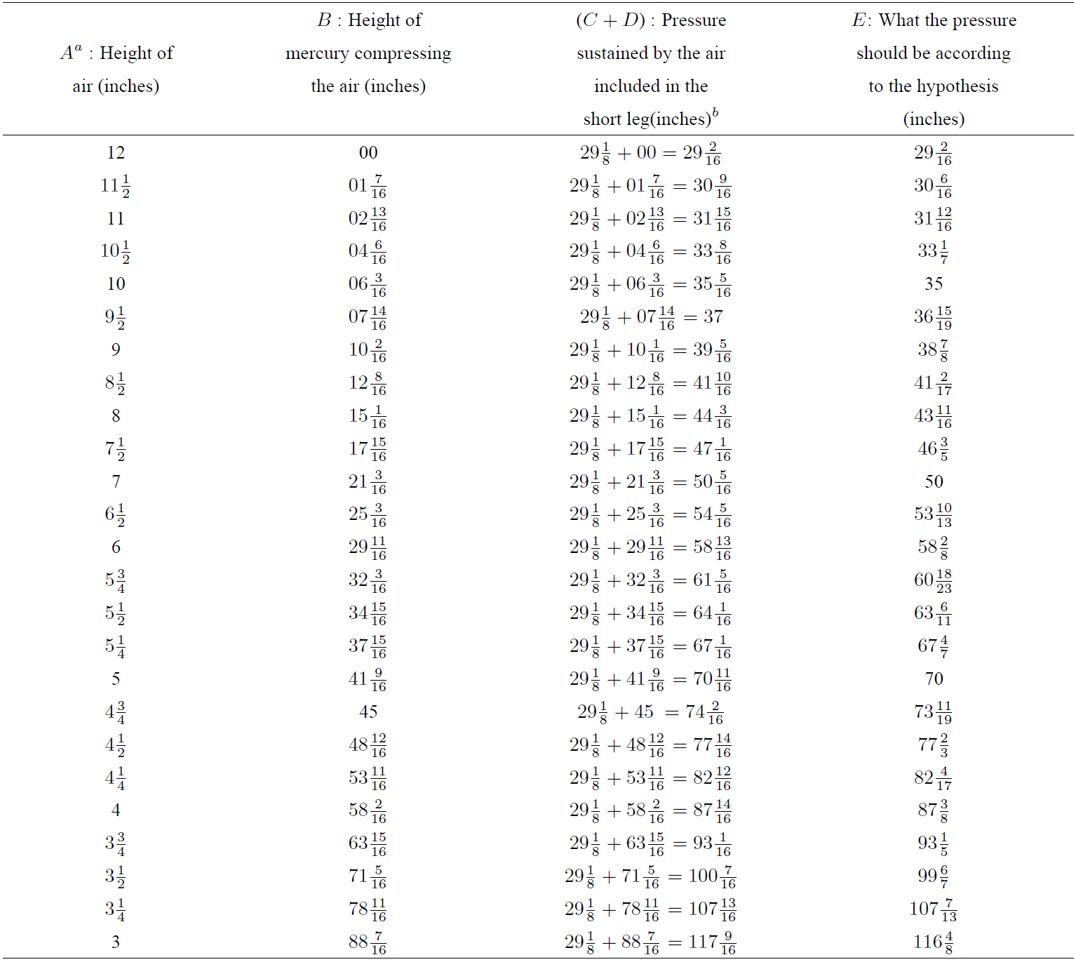
^aThe letters A to E are the same that are written in the original Table of Boyle’s book ⁶ to identify the data columns.

^bBoyle recorded in his experiment that the height of a mercurial cylinder that counterbalanced the pressure of the atmosphere was 29(1/8) inches; so, he added the value of 29(1/8) inches to every height observed in the longer leg in order to obtain the pressure sustained by the air, and this sum has been explicitally reflected in this table.

According to these results, Boyle concluded that his experiment provides sufficient proves about the reciprocal relationship between the volume and the pressure of the air: when volume of air is reduced to half its initial value, the pressure is near twice it was before; and when the volume is reduced again to half the previous value, the pressure is four times stronger than the initial pressure, although there is a positive bias between experimental pressure values and expected pressure values according to this hypotheses, as it can be seen in Table I. In Fig. 1 it is represented the evolution of this bias as a percentage of the expected pressure value when air is compressed from its initial equilibrium state.

Figure 1. Bias of the experimental pressure in Boyle’s experiment vs H air. 

3. Regression analysis of Boyle’s experiment data

Regression analysis is a powerful statistical tool to investigate the relationships between experimental data ^2,3,7. See Annex about teorical bases of linear regression model at the end of this article.

If we do a regression analysis of the Boyle’s experimental data shown in Table I ⁷, the following linear relationship can be obtained:

with a determination coefficient R ² = 0.9999 So, doing this regression analysis it is confirmed the reciprocal relationship explained by Boyle in his book between the volume, expressed in terms of height of air, and the pressure of the air ⁶. We have to take into account that the intercept obtained is an estimation of the intercept of the regression model, and an hypothesis test on the intercept shows that there is no statistical differences between the value obtained and zero ⁷:

Test on the intercept

b = 0

The value of the statistical t for the intercept is t = 1.599.

The critical value of the t-distribution for a 0.05 significance level and (25 - 2) degrees of freedom is t _0.025,23 = 2.069.

As 1.599 < 2.069 the null hypothesis for the intercept is accepted. So, there is no statistical difference between the value of the intercept of the regression equation and zero.

We can say then, that Eq. (2) is consistent with Eq. (1), taking into account that in Eq. (2) the volume is expressed in terms of height of air.

Analysis of the residuals gives a measure of the variability not explained by the regression model and residuals can be interpreted as the observed values of the errors ⁸. The residual plot presented in Fig. 2 shows another way of looking at the evolution of the experimental error in Boyle’s experiment, based on the regression analysis information. We can observe two zones; the first zone goes from the initial point to the point when the volume of air is reduced aproximately to half its initial value. In this zone it can be seen a pattern of autocorrelation ⁸. This can be caused by a presence of correlative error in the graduation marks of the tube and has been analyzed in the bibliography ⁹. The second zone shows an increase of the experimental error variability when the volume of air is reduced beyond half its initial value. The pattern of this second zone can be situated in an horizontal band between ±0.6 inches, showing a random experimental error that could have different origins; not controlled changes in temperature during experiment or some kind of not controlled practical aspects in measuring at the highest values of pressure.

Figure 2. Residual plot in Boyle’s experiment: (experimental pressure-pressure from regression model) vs H air. 

Under the assumptions of this regression analysis, from residuals knowledge we can do an estimation of the standard deviation of the experimental error:

and we can stablish a confidence interval for the estimation of the slope of the regresion model, that is; for the estimation of the constant for the reciprocal relationship between the volume of air (in terms of height of air) and the pressure (in terms of height of mercury) at the conditions of the experiment:

That means that the K value found has a relative uncertainty of 0.4%.

4. Discussion of results

In 1662 Robert Boyle made the experiment the results of which have been analyzed. Aproximately 200 years later, in the XIX Century it was established the ideal gas equation ¹⁰:

where: n: number of moles of gas R: universal gas constant T: absolute temperature of the gas

As we can see comparing Eqs. (1) and (3), the constant of the Boyle’s law is related to the universal gas constant R: The constant of the Boyle’s law is the value of R modified by the product of the number of moles n and the temperature T of the gas, at (nT) constant. So, we can write:

Therefore, a relative uncertainty of 0.4% in the value of K means a relative uncertainty of 0.4% in the value of R obtained in a reproduction of the Boyle experiment with (nT) known, constant and with negligible uncertainty.

As the accepted value of R¹¹ is:

this means that the uncertainty in R will be ±3·10^-4; affecting the fourth decimal number of R. This provides a prove about the great precision of the experiment that Boyle made in 1662.

5. Conclusions

An analysis of the original data obtained by Boyle in the experiment that he made in 1662 on the spring of air shows that, although there is a positive bias between the experimental pressure of the air and what the pressure should be according the hypothesis of reciprocal relationship between the volume and the pressure of air, the experimental error is low enough to estimate the constant of Boyle’s law with a relative uncertainty of 0.4%.

This means that a reproduction of Boyle’s experiment with (nT) known, allows to obtain from the ideal gas law an estimation of the universal gas constant with uncertainty in the fourth decimal of R, what indicates that Boyle made his experiment with a high degree of precision.