


 text new page (beta)
 English (pdf)
 Article in xml format
 Article references
 Send this article by e-mail
 Cited by SciELO
  Similars in
SciELO
Similars in
SciELO 
 Permalink
PACS: 78.67.Hc; 78.67.-n
1. Introduction
During the last two decades there has been an increasing interest toward the solution of different n-dimensional problems by meshless methods. This methods are referred as being applied over scattered data and independent of dimension. They have been found to be widely successful for the interpolation of scattered data. More recently, radial basis functions (RBF) methods have emerged as an important tool for the numerical solution of partial differential equations (PDEs) 1. RBF’s methods can be as accurate as spectral methods without being tied to a structured computational grid. This results in ease of application for the case of complex geometries in any number of space dimensions. This way of solution of PDEs has drawn the attention of many researchers in science and engineering.
One of the first meshless methods, the so-called Kansa’s method -developed by Kansa in 1990 2,3-, is obtained by directly collocating the RBFs, particularly the multiquadrics (MQ) one, in the look for the numerical approximation of the solution. Kansa’s method was recently extended to solve various ordinary and partial differential equations including the 1D nonlinear Burgers equation 4 with shock wave, shallow water equations for tide and currents simulation 5, heat transfer problems 6, and free boundary problems 7,8. In most of the cases, the accuracy of the RBF solution, however, depends heavily on the choice of the so-called shape parameter c in the multiquadric function ϕ(r) = (c2 + r2)β/2 or that for β in the Gaussian basis functions ϕ(r) = exp(-βr2). The choice of this optimal value is still under intensive investigation and many authors have investigated the role of this shape parameter. For instance, Carlson and Foley 9 have shown that it is problem-dependent. Tarwater 10 found that, by increasing c, the Root-Mean-Square (RMS) of the error dropped to a minimum and, then, increased sharply afterwards. In general, as long as c increases, the system of equations to be solved becomes ill-conditioned.
Radial basis function collocation is currently one of the main methods for meshless collocation. They differ from the polynomial basis functions typically applied in classical collocation methods. There are, in principle, two different approaches to collocation using radial basis functions. The symmetric approach relies on Hermite-Birkhoff interpolation in reproducing kernel Hilbert spaces 11 and its application to PDE was first analyzed in 12,13. The Asymmetric approach by Kansa 14 that will be used in this paper, has the advantage that less derivatives have to be formed but has the drawback of an asymmetric collocation matrix, which can even be singular in specially constructed situations 15,16. Despite this drawback asymmetric collocation has been used frequently and successfully in several applications. Schaback has shown that with some assumptions and modifications is possible to prevent numerical failure and to prove error bounds and convergence rates 16.
On the other hand, with the development of high-speed computing machines, seeking the numerical solution for the Schrödinger equation has become a subject of great activity. Analytic solutions for Schrödinger equation have been developed and studied extensively in past decades. In more than one dimension, the two main approximate techniques besides the direct solution of relatively few cases via special functions, are the perturbation theory and the variational methods 17. Many of the closed solutions have been established using these methods. However, in most cases the use of numerical methods is indispensable, for example, analytical solutions are not possible or become difficult to find in the case of an exciton in a spherical quantum dot system, due to the fact that the corresponding electron and hole effective mass differential equations cannot be uncoupled. Thus, it is important to find numerical alternatives for solving these equations that do not reveal as much demanding when it comes to computer capacity.
In recent decades, a rather large number of numerical methods have been developed for the solution of the Schrödinger-like problem. Among them we can mention the shooting methods 18,19; Anderson Monte Carlo 20; genetic algorithms 21; and variational methods 21, 22. Historically, the main approach for the numerical solution of the Schrödinger problem in more than one-dimension has made use of finite difference methods (to know about only a few of them see 23,24 and references therein). In recent times, some authors have put forward the use of the meshless approach for the solution of the Schrödinger problem in more than one dimension, as an alternative 25. Within the same spirit, the present work is aimed at providing some inside on the use of meshless algorithms for obtaining the eigenenergies and wavefunctions of one- and two-dimensional Schrödinger equations that can be related with the effective mass description of electron states in low-dimensional semiconductor heterostructures 26. We organize the article in the following way: In Sec. 2, we introduce meshless methods with the help of the concept of conditionally positive definite functions. In Sec. 3 we give details of the n-dimensional interpolation problem for scattered data. These tools are applied in section four in the numerical solution of Schrödinger eigenvalue problem by collocation of radial basis functions; we explain our algorithm and finally in section five we show the accuracy and application of our method comparing with some well-known analytical solutions of Schrödinger equation.
2. Meshless methods and Radial basis functions
The evolution of what is currently known as meshless methods started around 1950’s, closely related to spline theory, in the context of interpolation and approximation of functions 27,28, inverse problems 29,30 or computer vision30,32. Later, they have been applied to other problems, specially the numerical solution of PDE. Meshless methods are based on radial basis functions interpolators of the form S : ℝn → ℝ
where x and ai belong to ℝn , and ai are the interpolation nodes. Besides, ||⋅|| is the Euclidian norm and φ: ℝ → ℝ is a radial basis function. Some well-known choices for ϕ(r) are
Multiquadric
Thin Plate Spline (TPS) ϕ(r) = r2 log(r), and
Gaussian ϕ(r) = exp(-βr2).
On the other hand, p(x) is a polynomial term of small degree in n variables. For example, for thin plate spline in ℝ2, x = (x,y), and p(x) = β1+ β2 x+ β3 y. In some cases, S(x) does not have polynomial term as, for example, the multiquadric and the Gaussian radial basis. In accordance, we have the following
Definition 1 A function Φ: ℝn → ℝ is called radial if there exists a univariate function ϕ: [0,∞) → ℝ such that
where ||⋅|| is the Euclidian norm and ϕ is called a radial basis function(RBF).
In spite of the great number of available functions to be considered as radial basis, there is a relatively small number of RBFs that has arisen in the treatment of some particular problems, and constitute the commonly used radial functions in practice. They appear collected in Table I.

Given any function Φ : ℝn → ℂ, and a set of knots or centers 𝒜 =
{a1,…, aM} ⊂
ℝn , we can associate some kind of interpolation
matrix A, whose entries are Ajk
= Φ(aj
- ak), together with the quadratic form
Definition 1 A continuous function Φ : ℝn → ℂ is said to be conditionally positive definite (CPD) of order m on ℝn if
for any M different points 𝒜 = {a1, a2,...,aM} ⊆ Ω ⊂ ℝn and α = [α1, α2,..., αM]t ∈ ℂn , satisfying
for any p in Πm -1(ℝn). Where Πm-1(ℝn) is the ring of polynomials of n variables of degree less or equal than m - 1.
If αtAα > 0 -provided that the points ai are distinct- and α ≠ 0, we say that the function Φ is strictly conditionally positive definite of order m.
In particular, the case m = 0 yields the class of (strictly) positive definite functions. As a consequence of this definition a function which is CPD of order m on ℝn is also CPD of any higher order. Micchelli 33 showed that interpolation with strictly CPD functions of order one is possible even without adding a polynomial term.
3. The Interpolation Problem
Once the role of radial basis functions as interpolators is understood, the application for solving differential equations is straightforward. In order to properly illustrate, we first give a description of the interpolation issue. Accordingly, the approach to meshless reconstruction is based in the following multivariate interpolation problem:
Given a discrete set of scattered points 𝒜 = {a1,
a2,…, aM} ⊂
ℝn and a set of possible noisy measurements
{z1,…, zM} ⊂ ℝ, find a
continuous or sufficiently differentiable function f :
ℝn → ℝ, such that f
interpolates (f(ai ) =
zi) or approximates
(f(ai ) ≈
zi) the data
Example 1 Let us apply radial basis functions Eq. (1) to interpolate a surface
given in the form z =
f(x,y) from the data
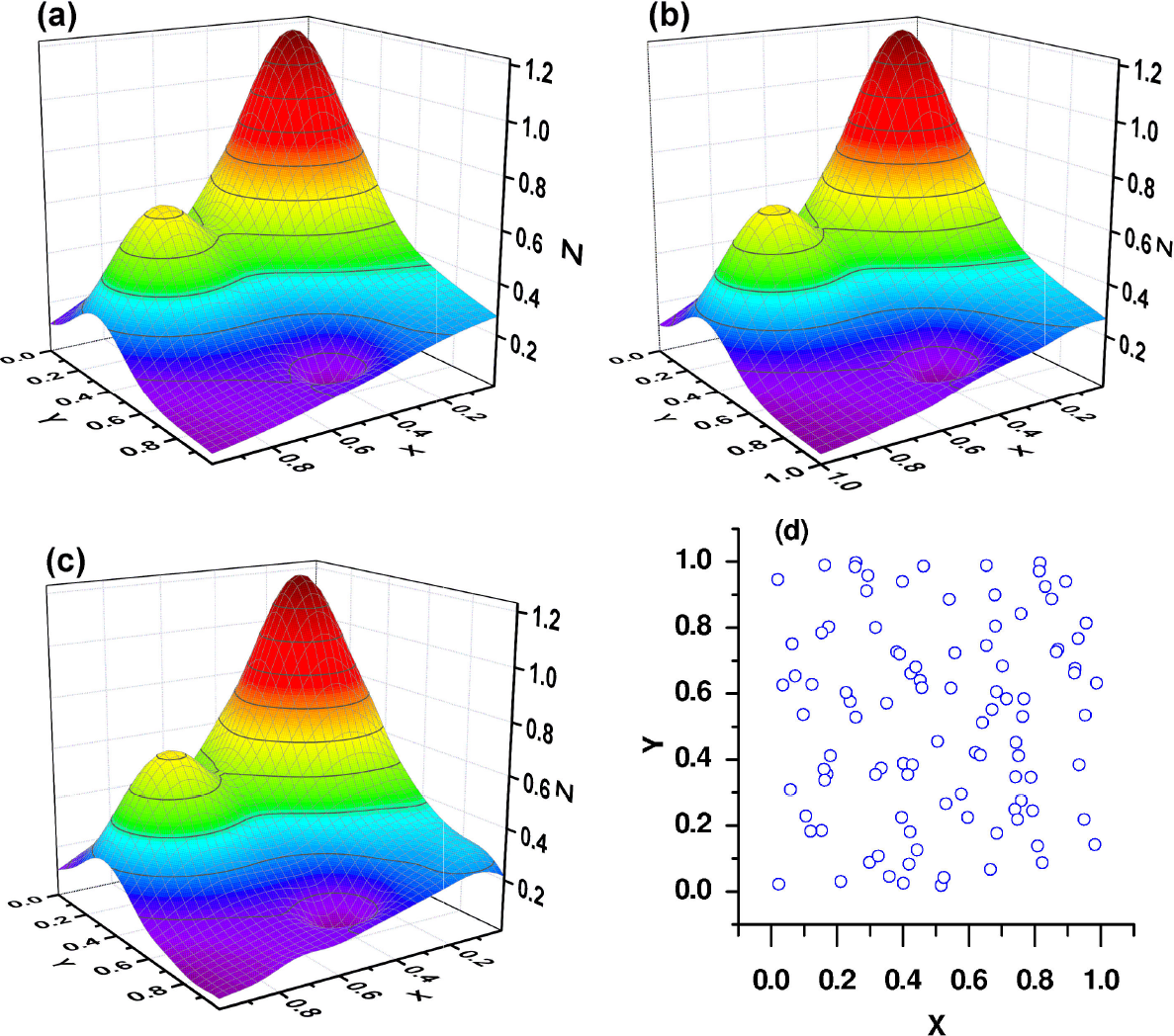
Figure 1 Reconstructions of Franke’s function: Direct plot of Franke’s function (a), Multiquadric reconstruction (b), Gaussian reconstruction (c), and distribution of the scattered points (d).
This function has been sampled for nodes in the region Ω = [0,1] × [0,1] (see Fig 1(d)) with M=100. The usual plot of f(x,y) appears in the Fig. 1(a), whereas applying the multiquadric and the Gaussian, S(x) -without polynomial term- to the scattered sample points, it has the form displayed in Figs. 1(b) and 1(c), respectively.
The interpolation conditions S(ai)=zi , i=1,2,…, M, produce M equations and the interpolant S is completely determined by the αi ’s after solving the system Aα = z, where A is an interpolation matrix, A = [Aij], with
It is possible to observe that the use of RBF interpolation in the reconstruction of the function leads to -essentially- the same graphics as it is were produced by the direct plot of the Franke’s function (in all cases we used MATLAB for producing the figures). Although the use of RBF interpolation in this example might be seen as useless, we consider it suitable for highlighting the power of this kind of interpolating schemes.
4. Meshless solutions of Schrödinger equation
As it is known, in quantum mechanics, the state of motion of a particle is specified by giving the wave function, which is -in general- the solution of the time-dependent Schrödinger equation. The Schrödinger’s equation (SE) is a postulate that constitute the fundamental equation of quantum mechanics. It affirms that the time evolution of a particle of mass m, described by a wave function ψ(x,t), is linked to the potential in which it is moving by the relation
In this partial differential equation
V(x,t) is the
local potential operator, which depends of the spatial position x =
(x, y, z) and the time
t. In addition,
-(ℏ2/2m)∇2 is the kinetic energy
operator, where ∇2
ψ = ψxx
+ ψyy
+ ψzz
is the Laplacian operator. The sum of these two latter terms defines what
is known as the Hamiltonian operator (or total energy operator)
The physical state of a particle at time t is completely described by the wave function ψ(x,t). The probability of finding the particle within a region Ω is
Since the particle must always be somewhere in the space, the probability of finding the particle within the whole space is one; that is, there is normalization condition that reads
Many interesting problems in quantum mechanics do not require considering the SE in its whole generality. Usually, the most interesting states of a quantum system are those in which the system has a definite total energy, and it turns out that for these states the wave function is a standing wave. In other words, the SE predicts that wave functions can form standing waves, called stationary states. When the time-dependent SE is applied to these standing waves, it reduces to a simpler equation called the time-independent SE,
The latter expression can also be written as an eigenvalue problem
It is generally accepted from the early stages of Quantum Mechanics foundation that the determination of the possible eigenvalues, E of the Hamiltonian characteristic Eq. ([eq:eigproblem]) is one of the essential problems of the study of the quantum world. Until today it has not been solved exactly for many physical systems. Even for relatively simple cases -some of which relate with the simulation of the energy band structure of artificially made condensed low-dimensional systems- the exact solution of the stationary SE is not possible with the means of nowadays mathematics. This constitutes a motivation for the use of efficient numerical approaches to obtain it; specially those capable of dealing in a handy way with 2D and 3D domains of complicated geometry. In this sense, it is possible to mention the application of a meshless approach by Dehghdan and Shokri 34.
Radial basis function collocation is currently one of the main methods for meshless collocation. They differ from the polynomial basis functions typically applied in classical collocation methods. There are, in principle, two different approaches to collocation using radial basis functions. The symmetric approach relies on Hermite-Birkhoff interpolation in reproducing kernel Hilbert spaces 11 and its application to PDE was first analyzed in 12,13.
The Asymmetric approach by Kansa 14 that will be used in this paper, has the advantage that less derivatives have to be formed but has the drawback of an asymmetric collocation matrix, which can even be singular in specially constructed situations 15,16. Despite this drawback asymmetric collocation has been used frequently and successfully in several applications. Schaback has shown that with some assumptions and modifications is possible to prevent numerical failure and to prove error bounds and convergence rates 16.
We now consider a general class of boundary or initial value problems for partial differential equations:
with 𝓛 a linear partial differential operator, and 𝓑 a linear boundary operator that prescribes values on the boundary of ∂Ω. If we look for a solution for 𝓛u = f such that
The collocation method finds an approximate solution to a differential equation evaluating in collocation points
is a system of linear equations. Then if we want to solve Eq. (13) with first order absorbing boundary condition
The Asymmetric Kansa’s approach assumes an approximate solution of the form
For NI
nodes
and
This leads to the matrix form
With
And the linear system we have to solve is
In particular, we are going to apply this scheme for solving the time-independent SE in ℝn(n = 1, 2) in the form of an eigenvalue problem with Dirichlet boundary conditions on Ω ⊂ ℝn
where
with N distinct collocation points 𝒜 = 𝒜Ω ∪ 𝒜∂Ω and ensuring (22) holds at these points. Evaluating (23) at the collocation points, we have a system of linear equations
Now, we introduce the notation ψj = ψ(aj ), ψ = [ψ1, ψ2,..., ψM , ψm+1,..., ψN]t , ϕij = ϕ(∥ai - aj ∥), and define the matrix
such that, according with Eq. ([duque]), it is possible to write
Here, A is strictly positive definite. So, it is nonsingular and we can put
On the other side A can be decomposed in two parts
and
Clearly, A = AΩ + A∂Ω. Hence, with (27) and the former notation, one obtains
where
As a result of this procedure, we finally arrive at
which represents the discretization of the eigenvalue problem associated to the time-independent SE (22).
From a purely mathematical point of view, the Eq. (22) can be solved for any value of the energy E and used to obtain a corresponding discretized wave function ψE (x). However, in the particular situation of allowed confined energy states, the wave functions are physically meaningful if they satisfy the boundary condition ψE(x) → 0 as ∥x∥ → ∞. So, we must check whether or not a solution obtained for some chosen value of E satisfies this asymptotic condition. In our algorithm this property is ensured by looking for solutions that are sufficiently close to zero at the boundary of the region Ω. That is, we require ||ψ∂Ω|| ≈ 0. In other words, we get physically acceptable wave functions ψE(x) only for a set of “allowed” discrete values of the energy, En (n=1, 2, ...). In accordance, ψE(x) is an eigenfunction of the SE, and E the associated energy eigenvalue.
4.1. The Algorithm
Now we briefly summarize the algorithm proposed for solving the SE in confined condensed
quantum systems. Typically, the Schrödinger problem in this kind of structures
involves the use of the so-called effective mass and parabolic approximations
which, under the assumption of independent energy bands, leads to the same
mathematical form given for the stationary SE in Eq. (8). INPUT. A
set of collocation points and the potential function
The following steps are:
Calculate matrix Aij= ϕ(||ai - aj ||), i,j = 1,..., N.
Calculate
Find eigenvalues and eigenvectors ψ = [ψ1, ψ2,..., ψN]t in Hψ=Eψ. Use an eigenvalues solver for non-symmetric matrices.
Among all eigenvectors ψ, to choose those which satisfy the boundary condition ||ψ∂Ω|| ≈ 0.
Calculate α = A-1ψ, α = [α1, α2, ...αN]t .
The eigenfunction or wave function is
5. Examples and numerical calculations
In order to show the advantages of the meshless approach introduced in this article we have made the choice of reproducing some pretty well known problems of quantum mechanics in one and two-dimensions. This will allow to compare with existing results, some of them showing analytical solutions. Thus, we leave the study of the energy states in less common structures for a future work. In all the following examples the inverse multiquadric RBF (β = -1) will be used.
Let us first address some of the simplest one-dimensional problems in quantum mechanics. It is worth mentioning that, although they might seem rather academic ones, their use as conduction and valence band bending profile models is pretty much extended in the literature on low-dimensional heterostructures. Among those that have direct analytical solutions we find:
Example 2 The one-dimensional harmonic oscillator.
The simple harmonic oscillator model plays an important role in many areas of physics. It is used in classical and quantum mechanics for a system that oscillates about a stable equilibrium point to which it is bound by a force obeying Hooke’s law F = -kx. Thus, any particle oscillating about a stable equilibrium point will oscillate harmonically for sufficiently small displacements. An important example of a quantum harmonic oscillator is the motion of ionic cores inside a solid crystal. Each atom has a stable equilibrium position relative to its neighbors and can oscillate harmonically about that position. Another important example is the diatomic molecule, such as HCl, whose two atoms can vibrate harmonically, in and out from one another. The quantum mechanical motion of the harmonic oscillator is described by the one-dimensional SE with potential energy function V(x) = 1/2m* ω2 x2 (Here, m* is the effective mass of the particle). The normalized complete set of eigenfunctions ψn(x) for the problem Hψ = Eψ can be expressed in terms of Hermite polynomials Hn(x) 35, 36. So we can write the Eq. (12), in this case, as
where ω is the cyclotron frequency.
The analytic eigenfunctions of the Hamiltonian above are given by
with the corresponding eigenvalues or energy levels
Here
We have compared these exact analytical solutions with the numerical solutions by meshless method (Table II and Fig. 2), the results obtained for the energy levels are in remarkably good agreement with the exact values.
Table II Eigenstates for the one-dimensional harmonic oscillator, given in units of ℏω, calculated with N = 500 collocation points. The CPU time was 13:1 s.


Figure 2 Eigenfunctions for the Harmonic oscillator potential. The confinement potential is shown by the parabolic line. Each wavefunction is localized on its corresponding energy. Energies and lengths are given in effective units. Used number of collocation points, N = 500. CPU time 13:1 s.
We define the effective Rydberg for the energy units [Ry* =
m* e4/(2 ℏ2
ε2)] and the effective Bohr radius for the length
units
Example 3 Particle confined in a finite double square quantum well (DSQW).
We now apply the meshless method with multiquadric basis function
where L1 and L2 are the widths of two square wells, which are separated by a potential barrier of length Ld . For the numerical evaluation we have used the effective units, defined above. In consequence, the problem to solve is given by the following differential equation
The calculated lowest eight confined energy levels as well as their corresponding wave functions are shown in Table III and Fig. 3, respectively. All the numerical procedure took 31 seconds of CPU time in an average portable personal computer, using MATLAB. The number of collocation points in the process was N = 500, where two of them were taken as boundary ones and another two were placed at the interfaces.
Table III (MM: Meshless method, DM: Diagonalization method) Lowest energy eigenstates of a finite
double square quantum well. On the second column there are the values
calculated by our algorithm. N = 500 interpolation
points were included in the calculation, with two of them taken as
boundary points. The remaining data are: L1
= L2 = 2:0


Figure 3 Schematic plot of the wave functions corresponding to eigenstates of a finite double square quantum well. Each wave function is placed at the energy corresponding to its eigenvalue. Details are the same as in Table III.
We turn to the solution of the SE in two-dimensional domains. In these cases, for the sake of simplicity, we choose systems with infinite potential barriers. However, this is not a restriction to the method provided finite potential structures can also be calculated by conveniently defining -as it turns out to be often in reality- a boundary ∂Ω, at which the condition of ψ(x) ≈ 0 fulfills.
Example 4 Schrödinger equation for a particle in an isosceles right triangle. The determination of energy levels and wave functions for a particle confined within different geometric structures in more than one dimension is relevant given the prospective use of these systems in modern technology.
There are some few cases with exact analytical solutions of the Schroödinger problem as it is the case of the one describing the motion of a particle inside a triangle. For a right isosceles triangle those solutions are given in the following conditions. In this two-dimensional problem there is a triangular infinite potential well that confines the particle inside a region determined by the length, L, of the two legs. Then it can be shown that the expressions for the eigenfunctions are 38,
for m = n ± 1, n ± 3,… and
For m = n ± 2, n ± 4,…
The corresponding energy levels, in effective units, are
The results obtained by our algorithm with N = 500 are in quite good agreement with the values obtained from the corresponding formula, (see Table IV).
Table IV Eigenenergies, in effective Rydberg units, for a particleconfined into a isosceles right triangle. Here the leg length is L = 4
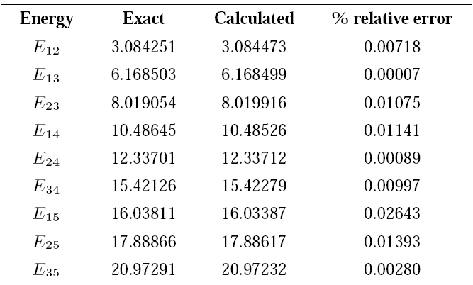
Figure 4 contains plots of the two lowest confined states obtained by solving the SE by meshless method and multiquadric RBF in the case of a right isosceles triangle with leg equals to
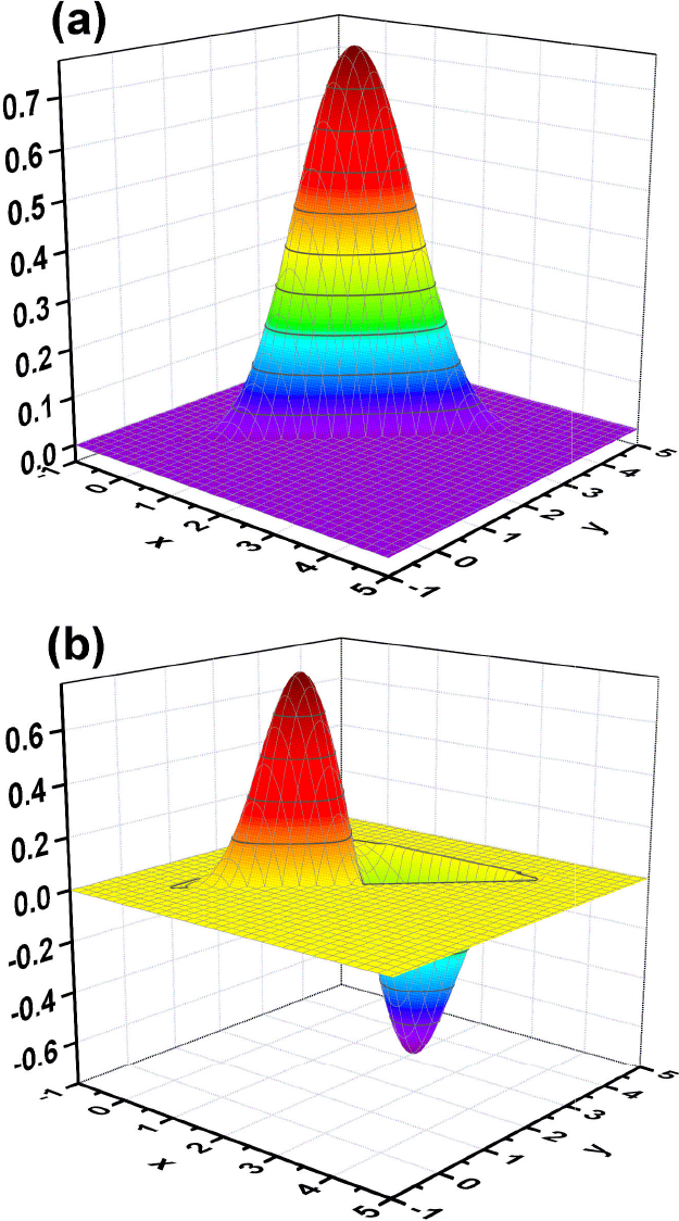
Figure 4 Numerical solutions for the wave functions of the two lowest energy states of a particle confined within a isosceles right triangle computed by interpolation methods 39, with data obtained using our algorithm. The scale is given in effective units.
The density plot of the wave functions of the calculated lowest eight energy eigenstates appear in the left-hand column of the Fig. 5, the corresponding densities of probability are shown in the central column.

Figure 5 Density plots for wave functions (left-hand panel) and their corresponding density of probability (central panel) associated to the first eight eigenenergies of a particle into a isosceles right triangle with infinite confinement potential. Density plot of absolute error between calculated and analytical density of probability for the first eight eigenfunctions (right-hand panel). The color bar in the bottom belongs to the right-hand panel.
On the other hand, right-hand column of the Fig. 5 shows the absolute error of the calculated solutions of the 2D SE equation, corresponding to the energy levels reported in Table IV, with respect to the exact analytical expression of Eqs. (35) and (36). We can see, in all cases, that the lack of coincidence is, at most, of the order of 10-2, with the higher accuracy being obtained for the lowest energy states. This is an indication that the numerical approach is pretty well accurate. In general the boundaries of the region present some difficulties to interpolants, since their reconstruction requires a precise spatial control over the smoothing properties of the radial basis function. Larger errors appear in regions close to the border triangle legs, and that is a consequence of a smaller density of points on the boundary and also of the global smoothness of radial basis interpolants.
Example 5 Particle in an infinite quantum disc.
The two-dimensional infinite quantum disc is defined by the confinement potential function
where r = (x2 + y2)1/2. Inside the disc region the well known analytical ψ(r,θ) functions that fulfill the boundary conditions ψ(r = R, θ) = 0 are given by using the Bessel functions, which depend on two independent integer quantum numbers m and n. They are given by (see 40 )
where Nm,n are the normalization constants, m = 0, ±1, ±2,… and km,n is the n-th zero of the function Jm(r), with n=1, 2, 3,…. Or, more conveniently, for bound states
and
with eigenenergies, in effective units, given by
The numerical results obtained by our algorithm are remarkably similar to the analytical
solutions, and are depicted in Table V for a
quantum disc of radius
Table V Eigenenergies for a particle into a quantum disc with infinity confinement potential. These values were obtained using N = 500 interpolation points within a disc of radius
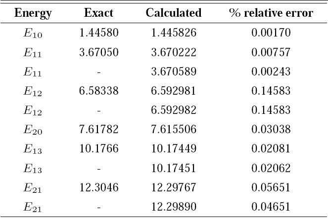
In the Fig. 6 we are presenting the density plots of the confined wavefunctions that correspond to the energy states reported in Table V (left-hand column) as well as the associated probability densities (right-hand column). It is possible to notice that the particular symmetries of the different states are correctly reproduced.

6. Conclusions and future research
We have addressed the subject of solving the Schrödinger equation in one- and two-dimensional problems using a meshless method. The procedure of implementing the numerical procedure has been thoroughly presented. For the sake of comparison, we chose some well known examples for the application of this approach which have, in general, analytical exact solutions. In all cases, the use of the meshless method leads to a remarkably good qualitative and quantitative agreement. In this paper we have used Multiquadric, a globally supported radial basis, the same as thin plate splines and many others. The main disadvantage of globally supported RBFs is that their associated interpolation matrix is full. As a consequence, there exists an upper limit in the number of collocation points of globally supported RBF collocation methods. If the distance between collocation points is very small, the matrix will become very ill-conditioned, leading to serious numerical singularity and degradation in numerical accuracy. These problems can be avoided by using compactly supported RBFs, and this is a subject of future investigation. That opens the possibility of using this kind of numerical schemes to the study of electron states -and related physical properties- in quantum nanostructures of more complicated or even non-regular geometries. Another possible application is the self-consistent solution of the Schrödinger and Poisson equations in problems with selective doping or polarization-induced charge densities.
A straightforward extension of our approach will be the study of quantum states in three-dimensional confined structures such as quantum dots. The results of such a work will be published elsewhere.

