1. Introduction

As students pass through their education at the undergraduate and graduate level, there is a need to develop skills in various disciplines; for instance, physics and mathematics are indispensable tools to address and generate practical solutions to current problems. Therefore, students must be able not only to analyze theoretical and technical solutions, but also to observe their relation to the context and other aspects of professional fields. Within this context, a linear systems course is presented as an excellent opportunity to integrate the acquired skills in the areas of physics and mathematics in order to design, model and simulate linear systems. A topic of high importance is the concept of state space resulting from the use of matrices.

It is important to use software tools that allow us to model and simulate such systems. Also, it is well known that the use of software as an alternative in the search of a particular numerical solution from a mathematical expression, is very convenient. Once we have used the concepts of physics and mathematics, as well as the technological resources through software, it is essential to continue all the way to the experimental realization; which leaves an unforgettable impression on students.

In this paper, we take a chaotic system that has the particularity of being linear in sections. The study of chaotic phenomena using tools from linear systems, gives students great skill in handling the matrix language, and on the other hand gives them the opportunity to deal with nonlinear systems.

In the last two decades, the study of chaos theory has been of great interest in mathematics, physics and engineering areas; the erratic behavior represented by mathematical models and their implementation across physical systems are studied. Generally, these systems are modeled by a set of nonlinear ordinary differential equations. In particular, one of the most widely studied systems is the Chua’s circuit ^1,2, considered as the transition from practice to theory. In other words, this system was the one that first hooked the attention of many researchers because in terms of theoretical development, it is relatively easy to physically implement different types of oscillators. One example is that different authors have shown that for linear systems attractors parts can be generated with multiscroll, as is the case of Suykens and Vandewalle ^3,4, where they introduced a family of n-scroll attractors. We decided to study the Chua’s circuit because it gives us the ease of having a linear piecemeal approach, where each part is a linear system.

To carry out the objectives mentioned above, some definitions and explanations (grounded mathematically) are given, to understand what is happening physically and theoretically. After being in context follows the study in detail of the Chua’s circuit from the equations of state, also we will show that it is easier to study this circuit with a similar matrix than with the original matrix.

Once the mathematical system is understood and solved, the next step consists in making the correspondent simulation with the help of a computer package. Later, details of the performed experiments are given, where the behavior of this circuit is documented ⁵. This work is structured as follows: in Sec. 2 definitions and theorems are given with their demonstrations. In Sec. 3, the mathematical model of Chua’s circuit is developed through Kirchhoff’s laws. In Sec. 4, the numerical solutions using the software Mathematica are shown as well as experimental results of the circuit, discussion and conclusions are exposed in Sec. 5.

2. Definitions and Theorems

In this section definitions of terms such as square matrix, eigenvalues, eigenvectors, matrix transformation, similar matrix, and some others are given, as well as theorems involving them. A good part of these definitions are developed numerically in Sec. 4.

Definition 2.1 We say that a square matrix A n × n is invertible (not singular) if ∃ other n × n square matrix B such that: AB = BA = I. B is called the inverse matrix A, denoted by A^-1.

Theorem 2.1 If the matrix A is invertible, then its inverse is unique.

Proof: Suppose A is invertible. B and C are inverses matrices of A, then B = IB = (CA)B = C(AB) = CI = C. As it demonstrated by the uniqueness of the inverse of A.

Definition 2.2 be a matrix A_n×m. Then Ker(A) = {x ∈ F^m : Ax = 0}

Theorem 2.2 If A_{n × n} is invertible, then Ker(A)={0}.

Proof: Let x ∈ Ker(A), then Ax = 0. Now A^-1 Ax = A^-10, the x = 0. It follows that in the kernel of A only can find the 0.

Definition 2.3 We say that a matrix A is similar to a matrix B if ∃ Q an invertible matrix such that: A = Q^-1 BQ where A, B, Q ∈ M_n×n (F)

Definition 2.4 A matrix A ∈ M_n×n (F) is said diagonalizable if this is similar to a diagonal matrix D.

Definition 2.5 be A ∈ M_n×n (F), an element non zero x ∈ Fⁿ is called eigenvector of matrix A if ∃ an scalar λ such that Ax = λx. Scalar λ is called eigenvalue corresponding to the eigenvector x.

Theorem 2.3 Let A ∈ M_n×n (F), then an scalar x ∈ F is an eigenvalue of A if and only if det(A - λI) = 0.

Proof: (⇒) Suppose that λ is an eigenvalue of A, it follows that ∃ x ∈ Fⁿ nonzero such that:

It follows that (A - λI) = 0 (because x is not zero) det(A - λI)x = 0 (applying determining both sides).

(⇐) Suppose det(A - λI)x = 0, it follows that the matrix (A - λI) is not invertible and thus ∃ x (nonzero) ∈ Ker(A - λI) such that (A - λI)x = 0, clearly Ax = λx and then λ is an eigenvalue of A associated with eigenvector x.

Definition 2.6 if A ∈ M_n×n (F), the polynomial f(t) = det(A - λI) is called characteristic polynomial of A.

Theorem 2.4 Let A, B ∈ M_n×n (F). If A is similar to B, then A and B have the same characteristic polynomial.

Proof: If we show that similar matrices have the same determinant, then the test is reduced to demonstrate that (A - λI) is similar (B - λI).

First is A ∈ M_n×n (F) similar to B ∈ M_n×n (F), then ∃ Q ∈ M_n×n (F) such that A = Q^-1 BQ.

Now the determinant of A is to be det(A) = det(Q^-1 BQ) = det(Q^-1)det(B)det(Q) = det(B) (since det(Q^-1) = 1/det(Q)).

We conclude that similar matrices have the same determinant. Let f(t) the characteristic polynomial of A and g(t) the characteristic polynomial of the matrix B. Then consider Q^-1 (B - λI)Q = Q^-1 BQ - λI = A - λI.

It appears that A - λI is similar to the matrix B - λI, therefore det(A - λI)=det(B - λI) this proofs that if A is similar to B, then A and B have the same characteristic polynomial.

Theorem 2.5 Let A be a square matrix and f(t) its characteristic polynomial. So

Proof:(a) (⇒) Suppose λ is eigenvalue of A, then ∃ x ∈ Fⁿ nonzero such Ax = λx. Then (A - λI)x = 0, it follows that (A - λI) is not invertible and that x is non-zero so det(A - λI) = 0 = f(λ) and thus λ is the root of f(t).

(⇐) Suppose it λ is a root of f(t), then f(λ) = det(A - λI) = 0. It follows that (A - λI) is not invertible so ∃ x ∈ Fⁿ nonzero such that (A - λI)x = 0. Then Ax = λx. That is, λ is an eigenvalue of A.

(b) f(t) is a polynomial of degree n, by the Fundamental Theorem of Algebra f(t) has n roots. It follows that A has at most n distinct eigenvalues.

Theorem 2.6 be A_n×n and be λ an eigenvalue of A. A vector ∈ Fⁿ is eigenvector of A corresponding to λ if and only if x ≠ 0 and x ∈ Ker(A - λI).

Proof: (⇒) Suppose that x is an eigenvector of A corresponding to the eigenvalue λ, then by definition x is not null and Ax = λx. Then (A - λI)x = 0, it follows that x ∈ Ker(A - λI).

(⇐) Suppose x is not zero and x ∈ Ker(A - λI), then (A - λI)x = 0, it follows that Ax = λlx and therefore x is an eigenvector of A corresponding to λ.

Definition 2.7 be A_n×n and is λ an eigenvalue of A. E_λ = {x ∈ Fⁿ : Ax = λx} = Ker(A - λI). E_λ is called the eigenspace of A corresponding to λ.

Given a linear transformation T: V → V, where V is a dimensionally finite vector space over a field K, this linear transformation is a matrix representation, and this matrix representation is obtained by applying the transformation vectors to a fixed base. Suppose that the basis of the vector space is β, and the matrix representing the transformation on that basis denoted by [T]_β , is a matrix in which the operations are not so simple. The problem lies in finding another basis β₁ of V such that [T]_β1 it is diagonal or block diagonal.

Any linear operator whose characteristic polynomial factors decompose in grade 1 there is a basis β for V such that

where J_i is a square matrix even if it is 1 x 1 in case the matrix is diagonal this matrix is called a block of Jordan, the matrix [T]_β = J₁ ⊕…⊕ J_k is called Jordan canonical form ⁶.

This is introduced because it is easier to work with diagonal matrices, if the matrix is known, it is implied that the linear transformation is also known and can be modified through this transformation matrix as carried out in modeling.

3. Modeling Chua’s circuit

Chua’s circuit (the simplest electronic circuit where a double scroll appears) is modelled in this section through the state equations:

Which form the internal representation, understanding that t is always present in the variables and for simplicity, we remove and rewrite the system as

Where A, B, C and D are matrices and let x be the vector column. Now it is time to introduce Chua’s circuit (shown in Fig. 1). A υ_m input was added to the circuit and taking as its output the potential υ₂ , the system can thus be interpreted through its state equations.

Figure 1 Chua’s circuit. 

The Chua’s diode has the skeleton shown in Fig. 2.

Figure 2 Chua’s diode. 

Now applying the laws of Kirchhoff of current and voltage, an internal representation model is obtained:

where

The latter equation gives the possibility of interpreting the Chua’s circuit as three systems, which are obtained when the

Diode 1 is on; when both diodes are not working and when Diode 2 is on, respectively. Then, the A matrix in (2) now is transformed in three A_i , where i = 1, 2, 3.

For example, if matrix A₁ is chosen, it’s obtained:

Here it becomes clear that the matrices B, C and D are the same in all three cases, the only changing matrix is A.

4. Numeric and Experimental Results

The equilibrium points that describe the system are found in this section, as well as the description of the two basins of attraction experimentally observed in Chua’s circuit. Before providing the numerical results, some definitions are cited, which will be validated by experimental results.

Definition 4.1 A pair (M, f^t) where f^t satisfies the properties of group and M is almost always a metric space is said dynamic system.

Definition 4.2 The set∪t=-∞∞ftx0 is called path or orbit for a given point x₀.

Definition 4.3 Let x ∈ M, F ∈ C¹ (differentiable) we assume that S is a topological sphere. D is called dissipation ball if:

Theorem 4.1 Two state equations {A, B, C, D} and {A¯, B¯, C¯, D¯} are equivalent zero state or have the same transfer function, ⇔D =D¯, CA^mB = C- A-m B¯, m = 0, 1, 2,…

See demo⁷.

Chua’s circuit is constructed with the parameters given in Table I.

Table I Values used in the Chua’s circuit. 

It should be specified that the below presented analysis consists on Diode 1 working (that is, only for A₁), since the process is similar to the other two cases. The software Mathematics 10.0 running on the Ubuntu-Linux platform was used to obtain the numerical values of the matrix A₁, its eigenvalues, eigenvectors, the transformation matrix P and the similar matrix. The obtained results are shown in Fig. 3.

Figure 3 Computed values using Mathematics 10.0. 

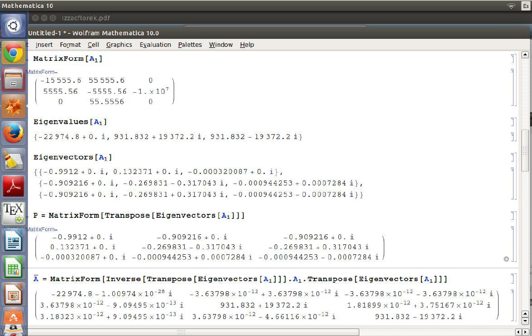
Note that using this software you can obtain the similar matrices by applying:

This way you are able to work with the similar system in its internal representation.

On the other hand, as a complement to the theory of linear systems, it is shown that the model used in this work is a chaotic circuit (see Fig. 4). In order to analyze this kind of systems, we have to find the equilibrium points of the dynamical system. Equilibrium points are obtained by equaling to zero the system (4) and replacing parts of the Eq. (5) concerned; it is assumed that the system has no entry (i.e.) in Fig. 1, V_m = 0. If the calculations are carried out, the following equilibrium points are obtained:

Figure 4 Experimental circuit of Chua. 

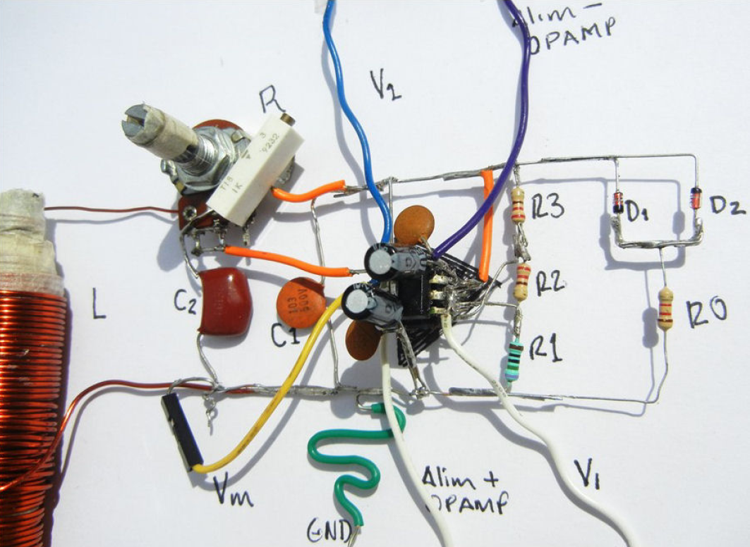
Figure 5 illustrates the ball of dissipation of the system, in this case it is a topological circle. In other words: for any given point x₀ in the xy plane there exists a number t > 0 such that A^t(x₀) = A(A(A(...(A(x₀))))) forms a path that goes into the ball of dissipation. Once inside it, it cannot go out and it is confined to oscillate between the points of balance, where A is the matrix system. See demonstration ⁸.

Figure 5 Phase portrait of dissipation Ball. 

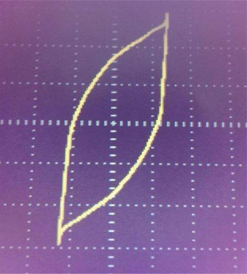
Figure 6 depicts a phase delay of the equilibrium points, which behave as attractors and repulsors. Even if the number of oscillations is enormous, the system will never leave the dissipation ball. Mathematically, this situation has a starting point and the number t > 0 is small.

Figure 6 Phase portrait with two attractors. 

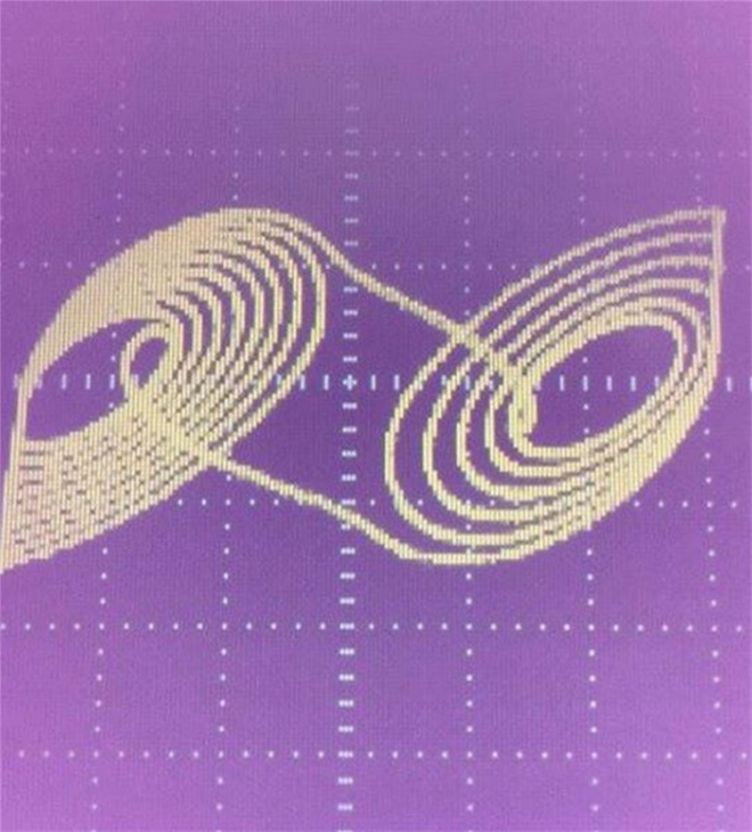
For Fig. 7 the number t > 0 is large enough to generate sufficient oscillations.

Figure 7 Phase portrait for t → ∞. 

Figure 8 illustrates the case when the system is only able to orbit in one attractor, and it does not have the necessary amount of energy to leave one attractor and go to the other.

Figure 8 One attractor. 

5. Conclusions

Different software tools can be used to find the solution of the matrix equations. In this paper, we used Mathematics 10.0 running on the Ubuntu-Linux platform. Matlab can also be used to solve this sort of problems, however, neither Mathematics 10.0 nor Matlab are open access utilities, hence their purchase requires an investment, making it difficult for students to use on their simulations and models. Luckily, freely distributed options are available, packages like Octave and Scilab software can be used as auxiliaries in teaching physics and mathematics.

Another important point of this work is the agreement of the experimental results with the theoretical predictions. This fact is very appealing to students, since the application of theory on real-life problems adds great value to their development as professionals.

As future work, we will attempt to mask an information signal through this circuit using the potential υ_m marked in Fig. 1, which could be used on signal-processing related issues.