1. Introduction

The equation of state introduced by van der Waals (vdW) in his doctoral dissertation, in 1873, was the first in a family of so-called cubical equations of state proposed with the aim of providing a better description of thermodynamic systems. One of the most important advantages of these equations is that they allow us to study phase transitions and the behavior of the system around the critical point. On the other hand, a relatively simpler equation of state can be obtained using results from the theory of ensembles and a simple interaction potential. Considering, for example, a fluid of hard spheres with a Yukawa tail (HCY), it is possible to obtain analytically the thermodynamic properties in terms of the parameters of the potential. For the particular case of an HCY potential, the MSA provides an analytical expression for the radial distribution function. This function is the basis of the integral equation theories (IETs) of the modern theory of fluids. The original MSA solution for the HCY potential, due to Waisman ¹, is analytic but not explicit. Hoye and Blum et al. ^{2, 3} obtained analytic results for the thermodynamic functions. Ginoza ⁴ simplified this solution but his results are not quite explicit. Perturbation theory has been very useful to obtain explicit expressions ⁵. The procedure devised by Tang and Lu ⁶ allows to obtain analytical expressions for the first-order term of the radial distribution function. Henderson et al.^{7, 8} proposed a perturbation approximation and they found analytical formulas for the energy and the pair correlation function at contact up to fifth order in the inverse temperature for an attractive HCY. The approach used by Henderson has also been extended for the case of a repulsive HCY ^{9, 10}. The thermodynamic properties obtained by Hoye et al. ^{2, 3} and Henderson ^{7, 8} are written in terms of a parameter satisfying a polynomial equation. Different methods, like the iterative method ¹¹, which is the most used, and the series inversion method, may be used to find the physically acceptable roots for this parameter ^{17, 8, 12}.

In this paper, we will show the methodology used to deal, on one hand, with a cubic equation and, on the other, with an equation obtained within the MSA, using only the inverse temperature expansion to find the physical root. We use both equations to predict the behavior of argon and the analytical results are compared with recent experimental measurements.

2. Cubic Equations

Recently, a general cubic equation of state, which we will call the Guevara equation, was proposed. It may be written as ¹³:

where T is the absolute temperature, p, the pressure, and ῦ, the molar volume of the system. Additionally, there appear, in these expression, three parameters, b, c and d, and a temperature function, a(T). This function, in turn, may be expressed as a cubic polynomial in the volume:

It is known that, for the set of values (p_c , υ_c , T_c ) defining the critical point, cubic equations of state have a unique, triple, real root, and, because of this, the Guevara equation may be written as a cubic polynomial in the volume:

Evaluating Eq. (2) in T = T_c and o = p_c and equating it, term by term, with Eq. (3), we obtain a set of three equations involving the three parameters, b, c , and d, from where it can be found that ¹⁴:

Where λ = (ξη)^1/3, η = RT_c /p_c , and ξ = a(T_c )/p_c . Notice, from the expressions for c and d that they are conjugate binomials. Taking advantage of this symmetry, the term (ῦ - c) (ῦ -d) can be written in a very particular form. To do it, let us first define the following auxiliary parameters:

Using them, Eqs. (5) and (6) become:

Introducing these parameters into (ῦ - c) (ῦ -d), we get

where υ ≡ ῦ - ωυ_c . Notice also that using Eqs. (4) and (7), the term ῦ - b can be expressed in terms of υ, as

where νυ_c ≡ (3/2)λ-η. Thus, Eq. (1), which originally was written in terms of three constant parameters and one temperature function, is now written in terms of only two constant parameters, ν and τ, and one temperature function, as:

or, solving for the pressure,

An important element to consider in Eq. (12) is the parameter a(T), which cannot be determined in a formal way and, consequently, it has been defined empirically in different ways. A simple way to obtain a(T) is writing Eq. (1) in the form of the virial equation and comparing the terms of one equation with the terms of the same density power of the other. One finds that ¹⁴:

Since the second virial coefficient can be measured in experiments, the value of a(T) may be found immediately. However, from the point of view of statistical mechanics, the second virial coefficient depends on the interaction potential being used. As this could be the square well potential or the Lennard-Jones potential, among others, there will be different expressions for a(T). For example, for the square well potential one has ¹³:

from where, an expression for a(T) is found as:

In this way, the equation of state has been completely specified. We can rewrite Eq. (12) in terms of dimensionless variables by introducing the reduced parameters υr≡υ/υc, pr≡p/pc, and Tr≡T/Tc. We obtain:

where α3(Tr)≡a(T)pc/R2Tc2 ¹³. Comparing with the reduced Guevara equation,

it may be seen that we have reduced the denominator of the second term on the right hand side of the equation. This shows that the equation does not depend on three parameters, but only on two.

3. Coexistence Curve

The construction of the coexistence curve is a direct application of Maxwell’s equal-area rule. This curve encloses the region where the phase transition occurs, i.e., the region where the liquid and gas phases coexist. To construct this curve, and in order to simplify the calculations and to find the values of the parameters involved, it is convenient to use a reduced or dimensionless equation of state. We use a numerical method implemented through a computer program that, in principle, can process any reduced cubic equation to find the coexistence region for the liquid and gas phases at different temperatures. The program finds a set of points that, taken together, form the coexistence curve.

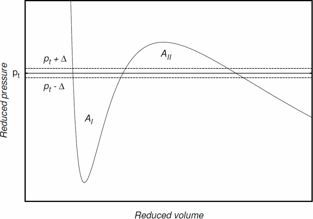
To exemplify how the program functions, it was applied to find the coexistence curve for Eq. (1). Essentially, the program finds the roots of the reduced equation for different isotherms. For a given isotherm, these roots are the intersections of the isotherm with the straight line representing the constant pressure at which the phase transition occurs. Notice that the value of this pressure of transition will be within the interval limited by the minimum and maximum of the isotherm. These extrema can be found from the expression for the reduced pressure, Eq. (17), by imposing the following condition:

To find the roots, this condition may be written as a polynomial in the reduced volume, as

In this particular case, the starting expression is cubic in the reduced volume, while, after equating its derivative to zero, a fourth order polynomial in the reduced volume is obtained. This suggests that, from a total of four roots, at least two must be real and must represent the reduced volumes for the minimum and maximum of the isotherm. It may be seen from Eq. (17) that p_r < 0 for υ_r < B, which corresponds to non physical systems. For this reason, one searches for roots of Eq. (19) satisfying the relation υ_r < B. It is found in general that B > 1/3; therefore, the physically meaningful roots must be greater than 1/3 ^13,14.

Using the bisection method ¹⁵, we look for the first two roots vr1 and vr2 satisfying υr1,υr2>1/3. It may be expected that these are the reduced volumes corresponding to the minimum and maximum of the isotherm; then, the mean point between these volumes vr3≡(υr1+υr2)/2 is found and an approximation for the pressure at which the phase transition occurs is proposed as pt≡p(υr3). The straight line p = p_t intersects three times the isotherm at three values of the reduced volume which correspond to the roots given by Eq. (17):

Writing this equation as

one obtains a cubic equation in the reduced volume; its roots are found using again the bisection method. Let these roots, ordered in increasing value, be a₂, b₂, and. c₂ After obtaining them, one proceeds to verify if, using these roots as integration limits, the two regions enclosed by the isotherm and the constant pressure straight line satisfy Maxwell’s equal-area rule, i.e., if the following equality is true:

Our program evaluates integrals, approximately, by means of Riemann sums. For the areas represented by the left-hand side and right-hand side integrals in the last equation, the approximated values A_I and A_II , respectively, are calculated ¹⁶. They are then accepted as equal if they satisfy the following criterion:

If it is found, in this first approximation step for p_t , that the absolute value of the difference between the areas is greater than the chosen error ϵ = 10^-4, then, according to the criterion, Maxwell’s equal-area rule is not satisfied, and one has to propose a new value for the transition pressure.

Thus, as a next step in the approximation, if A_I < A_II , the line of constant pressure is shifted by a a certain positive definite quantity Δ, i.e., a new value pt'=pt+Δ for the transition pressure is proposed. On the contrary, if A_I > A_II , the proposed new value is p_t = p_t - Δ. In this way, the size of the region having lowest area is increased, and the size of the other, decreased, as an attempt to obtain new areas fulfilling the criterion given by Eq. (23). This can be seen in Fig. (1). After shifting the line of constant pressure, the bisection method is used again to find new roots, a2',b2', and c2', and, with these, new values for the areas, AI' and AII', are calculated. And so on and on, until the absolute value of the difference between the areas is less than ϵ.

Figure 1 Shift of the line of constant pressure p_r = p_t for the reduced temperature T_r = 0:9. 

Applying this algorithm to different isotherms, it is possible to obtain sets of data {pi,υi1,Ti} and {pi,υi2,Ti}, which comprise, for each value of the reduced temperature T_i , the transition reduced pressure p_i and the reduced volumes υi1 and υi2 of the two coexisting phases. These sets represent points of the coexistence curve and, using them, leaving outside T_i , we may represent this curve in a P-V diagram, or, leaving outside p_i , in a T-V diagram.

This method may be used for any reduced or dimensionless equation provided that all the constant parameters defining the equation are known.

4. Equation of state and chemical potential for a Yukawa-type fluid

The modern statistical mechanics of fluids is based on the calculation of distribution functions or correlations functions, which describe the average structure of the system. The main question to be answered in this formalism is: Given the intermolecular potential between the molecules in the system, what will be the structure of the system at a given thermodynamic state point? Usually it is assumed that the intermolecular potential is pair-wise additive, with the consequence that, to describe all the thermodynamic properties of interest, only the pair structure is needed. Although the assumption of pair-wise additivity is not valid at high densities and low temperatures, it proves to be good in most instances. An important equation relating several correlation functions, which is the basis of the integral equation theories (IETs), is the Ornstein-Zernike equation. For homogeneous fluid, this equation is expressed in the form ^{5, 17}

where h(r) is the total correlation, and c(r) is the direct correlation function. The IETs are based on solving the Ornstein-Zernike equation, for which an additional equation, the closure condition, is needed. However, unlike the case of molecular simulation, the IETs necessarily involve approximations and consequently their results are not exact. For this reason, they are frequently referred to as integral equation approximations (IEAs).

IEAs can play an important role in the formulation of semi-empirical equations of state by providing the theoretical basis and functional form for equations of state which can then be used to correlate experimental data. The Ornstein-Zernike solution from the MSA closure condition enables us to readily obtain thermodynamic and structural properties, such as the radial distribution function, g(r) = h(r) -1, and hence the total energy ^{5, 17}:

Then, the equation of state can be written as:

where k_B is the Boltzmann constant, ρ is the number density, and N is the number of particles. Finally, u(r) is the intermolecular potential.

The HCY fluid is a model for a simple fluid that consists of hard spheres with a Yukawa tail. Therefore, the interaction between the gas particles is modelled by ¹⁸:

where σ is the diameter of the particles, r, the average distance between them, z, the inverse of the potential range, and ε, the amplitude of the attractive interaction between the gas particles. One feature of the HCY model is the possibility of changing the range of the interaction by varying z.

The MSA assumes that direct correlations are proportional to the model potential, and, consequently, for the Yukawa-type interaction model, one obtains explicit expressions for the thermodynamics, i.e., the compressibility factor for a single component gas is written as ^{2, 3, 11, 19}:

where Z(HS)=ϕ1+ϕ+ϕ2-ϕ3/Δ3 is the compressibility factor for a gas of hard-sphere-type particles, ϕ=πρσ3/6 is the packing fraction for N spherical particles contained in a volume V = N/ρ, and Δ = 1 - ϕ.

Within the MSA, the value of K is related to the inverse of the temperature, K = ε/k_BT, where k_B is the Boltzmann constant. Also, within the MSA, the chemical potential in dimensionless units, is written as ^{3, 20}

where the chemical potential of an ideal gas is given as:

Here, k_r and ϕ_r are quantities of reference, and the hard-sphere chemical potential has the following mathematical form ²¹:

Finally, the remaining quantities appearing in the above equations are defined in Appendix A.

Solutions for the thermodynamical quantities, within the MSA, for the interaction model given by Eq. (24) are obtained once the value of the accumulation parameter Γ = Γ(T,ϕ,z,ε) is known. This parameter is obtained through the series expansion of the inverse of the temperature, i.e. ^{7, 12},

The expressions for the coefficients of this series are given in Appendix A.

5. Coexistence Curve for a Yukawa-type fluid

The value of the inverse of the potential range has been taken as zσ = 1.8, which is the most appropriate for noble gases or Lennard-Jones system ¹⁸. The value of the interaction amplitude ε has been set so as to reproduce the experimental value of the critical temperature, T_c ≈ 151 K for argon^{17, 18, 22, 23}. The critical state (or critical point) (T_c , ϕ_c ) for the liquid-vapor transition is obtained from the compressibility factor. In the critical point, the compressibility factor as a function of reduced volume or density has an inflection point, i.e., the following condition must be satisfied:

In this way, the value obtained for the interaction amplitude is ε/k_B = 122 K and it allows us to determine the experimental critical point for argon as (T_c , ϕ_c ) = (151.3 K, 0.167).

Now, to obtain the liquid-vapor coexistence curve for argon, one may use the Gibbs-Duhem equation. This is a relation between changes in the chemical potential of the components of a thermodynamic system and changes in the pressure or in the compressibility factor μ(Z).The liquid-vapor coexistence curve encloses the region where the liquid (L) and gas (G) phases coexist in thermal equilibrium, i.e., at equal pressure and temperature, both phases will have the same chemical potential, that is, μ^L (p,T) = μ^G (p,T). Then, using Eqs. (25) and (26) we obtain the functional relations that allow us to determine the values of the frontier states where both phases coexist, i.e., μ^L (Z,T,ϕ^L) = μ^G (Z,T,ϕ^G), where ϕ^G < ϕ_c < ϕ^L . For a isotherm, the values of μ^L and μ^G that are in the coexistence curve are accepted with a tolerance of |μ^G - μ^L | < 10^-4.

6. Results

The coexistence curve for argon was constructed in two ways. First, in a thermodynamic approach, using a cubic equation of state, and second, within the MSA, considering a monodisperse gas with a hard-sphere plus a Yukawa-tail interaction. The results were compared with recent experimental data for Ar. In 1945, Guggenheim ²² collected a great quantity of experimental data for different systems and, from them, he constructed coexistence curves in the T - ρ (reduced temperature versus density) diagram. More recently, in 1994, Gilgen ²³ reported carefully measured values to construct the same diagram for argon. We have successfully constructed the coexistence curve in the T_r - ρ_r diagram for Eq. (12) using Padé approximants (Appendix B) and data reported for argon. We obtained, with an error of less than 0.01%, the following approximation ¹⁴:

The error estimated is the mean quadratic error (MQE); this gives a very precise result for the Padé approximant which allows us to work directly with the appropriate Padé approximant for each set of values of coexistence curves.

On the other hand, we were also able to obtain enough information to construct the phase diagram for argon. Putting together the three phase diagrams (for the Guevara equation, the Yukawa-tail approach, and the experimental data) it is possible to get a clearer comparison of the equations of state, as it may be seen in Fig. (2).

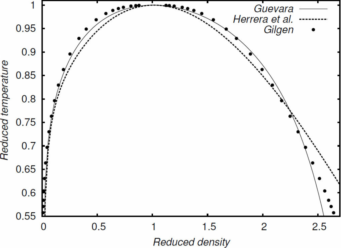
Figure 2 Coexistence curves for argon. The solid line was found from the Guevara equation ¹³, the dashed line from the MSA approach (Herrera et al.) ^13,14. The points are experimental results reported by Gilgen ²³. 

Notice that both, the theoretical scheme of the MSA and the use of the second virial coefficient in the equation of state, predict correctly the experimental results, particularly for low and medium densities; however, for high densities, there exists some discrepancy.

It is worth mentioning that, using the thermodynamic method, coexistence curves for carbon dioxide, ethane, and nitrogen were also obtained. In all these cases, our results are in very good agreement with experimental measurements ^{14, 24-26}.

In the case of an MSA closure, the HCY potential has been frequently parametrized to obtain good agreement with computer simulation results ¹⁸. The same good performance is obtained with perturbation theory in the MSA, both for attractive and repulsive HCY potentials ^{9, 10, 27}. Further, our theoretical results have been applied to find the static structure and the thermodynamics for krypton, obtaining good agreement with experimental data ²⁸. The equation of state and the chemical potential within the MSA correctly predict the critical state and the coexistence curve for low and medium densities, because the model used is similar to the Lennard-Jones potential, but with adjustable parameters, such as the amplitude of the attractive interaction, which we have adjusted to predict the experimental critical point for argon ^{17, 23}. Thus, the effects of three-body forces may be regarded as included in the effective potential. However, for high densities there is a discrepancy because the MSA does not take into account the real intermolecular potential for argon. As a matter of fact, the MSA and the IETs, in general, are unable to reproduce correctly the properties of liquids. As a consequence, the MSA does not describe equally well a rather dilute system and a dense fluid with well developed short-range order.

7. Conclusions

Along this work we have studied the predictions of two equations of state. In one hand, a general cubic equation of state that is able to represent the thermodynamic properties of the system by requiring parameters characterizing each system, which may be obtained experimentally. This equation predicts a phase transition between the liquid and gas states and an analytical expression can be obtained by means of a computer program based on Maxwell’s equal-area rule, and also by the method of Padé approximants. On the other hand, an equation obtained using the MSA, which includes information about the molecular properties of the system. This equation predicts also the liquid-gas phase transition, and the coexistence curve can be constructed by remembering that the chemical potential satisfies, through the transition, a condition of equilibrium, which is the analogous of Maxwell’s construction. Both equations succeed in providing a correct prediction for the coexistence curve at low densities; for high densities, however, there exists a noticeable deviation, as it could be expected, since, in the case of the cubic equation of state, the virial approximation is used only up to second order, which is adequate for the treatment of low density systems; for further detail it is necessary to consider virial coefficients of higher order. While in the case of the MSA treatment, the model used for the interaction potential and the chosen size of its range constitute a limit in the correct representation of the interaction between particles.

Both equations, even if one reflects macroscopic, and the other microscopic, characteristics of the system, lead to the same behavior, which in this case is the phase transition, and their results are very similar and in very good agreement with experimental data for argon. This confirms the correctness of the relation between statistical mechanics and classical thermodynamics. The methodology used in this work can be used for the treatment of other systems, and the curve of coexistence for other systems can be constructed through the computer program. For a given cubic equation of state, the coexistence curve can be constructed in any of the possible diagrams of the variables (p, V, T), and it may function, in a general way, as a reference to exhibit the transition between the gas and liquid phases. Further, it was possible to show that the method of Padé approximants is a very precise (precise enough) and that it may be used for any set of data (x_i , f_i) obtained from experiments.