


 nueva página del texto (beta)
 Inglés (pdf)
 Artículo en XML
 Referencias del artículo
 Enviar artículo por email
 Citado por SciELO
  Similares en
SciELO
Similares en
SciELO 
 Permalink
PACS: 51.20.+d; 66.10.Cb; 36.40.Sx; 68.35.Fx
Thermal waves (TW) are temperature oscillations resulting from periodical heating of a material1. They are often described as the solutions of the parabolic heat diffusion equation (PHDE) in the presence of a periodical (sinusoidal for a sake of simplicity) time varying heat source modulated in intensity at a given frequency, f1.
Consider an isotropic homogeneous semi-infinite solid, whose surface is heated uniformly (in such a way that the one dimensional approach used in what follows is valid) by a source (light, for example) of periodically modulated intensity (Io /2) Re[(1+exp(iωt))], where Io is the intensity of the light source (energy per unit area and unit time), ω is the angular modulation frequency, t is the time, i =(-1)1/2 and Re denotes the real part.
The temperature distribution T(x,t) within the solid with thermal diffusivity α can be obtained solving the (parabolic) heat diffusion equation (PHDE) 1,2
with the boundary condition
where k is the thermal conductivity, related to the thermal diffusivity, α through
Here ρ is the density and c is the specific heat at constant pressure.
The condition (2) express that the thermal energy generated at the surface of the solid (for example by the absorption of light) diffuses into its bulk by diffusion. It is supposed here that all the deposited energy is transformed into heat. From now on, the operator Re() will be omitted, taking into account the convention that the real part of the expressions of the temperature must be taken to obtain physical quantities3.
The solution of the problem with interest for practical applications 1 is the one related to the time dependent component. If we separate this component from the spatial distribution, the temperature can be expressed as:
Substituting in Eq. (1) we obtain
where
and
The general solution of the above problem is then
where
Expression (8) has the meaning of a plane wave. Like other waves it has an oscillatory spatial dependence of the form exp(iqx), with a wave vector q given by Eq. (6). Because it has several wave-like features, Eq. (8) represents a thermal or temperature wave (TW). The detection of TWs is the basics of the so-called photothermal techniques that have gained in interest since the early 1970s due to their potential not only for optical spectroscopy, but also for the measurement of thermal properties of materials 1. Although the main properties of TWs have been discussed in detail by several authors, this work will be focused on one of their main properties, namely the propagation velocity.
From Eq. (8) it is easy to see that TW’s wave-length is given by λ = 2πμ so that they propagate with phase velocity, Vp , given by:
As in other wave phenomena, the phase velocity is defined as the velocity of points of constant amplitude in a wave of the form given by the above expression. Since Eq. (5) is a linear ordinary differential equation describing the motion of a thermal wave, then the superposition of solutions will be also a solution of it (we have approximated the temperature distribution by just the first harmonic of that superposition because the higher harmonics damp out more quickly due to the damping coefficient increase with frequency). This superposition represents a group of waves with angular frequencies in the interval ω, ω + dω travelling in space as “packets" with a group velocity:
where qR = Re(q) = 1/μ. This velocity is the phase velocity of the envelope, i.e. the velocity at which thermal energy propagates. In other words, it is the velocity of points of constant amplitude in a group of waves and is calculated from the dispersion relation (Eq. (6)) as usual.
The group velocity is twice the wave’s phase velocity 2. If TW are truly waves, then this velocity must be smaller than the light speed in vacuum, 3 × 10⁸ m/s, otherwise one of the postulates of the special relativity theory will be violated. Therefore, in order to keep
the following condition must be achieved
which is obtained after substituting Eq. (10) into Eq. (11). The frequency fc will be called here the critical frequency.
Values of fc for different materials (with different α values) are given in Table I. For example, for a poor heat conductor such as balsa wood (α = 0.5 × 10⁻⁷ m2/s) the maximal available frequency is about 1022 Hz. For frequencies values higher than fc the group velocity becomes larger than c. Thus, it can be concluded that for each material a critical frequency, fc , exists above which heat cannot be modulated, otherwise relativity theory can be violated. This is a result that contradicts any experience because there is not a technical upper limit for the modulation frequency. In other words, frequencies given by Eq. (12) can be easy exceeding in practice. Therefore, for these frequencies Fourier treatment of heat transport becomes inadequate.
Table I Values of thermal diffusivity, second sound velocity (Eq. (14)) and the critical frequency (Eq. (12)) for some solids materials. The used value of τ is 10-12 s. Thermal diffusivities were taken from: http://www.fiz-chemie.de/infotherm/servlet/infothermSearch (downloaded March, 2015)
| MATERIAL | α (m2/s) | fc (Hz) | u (m/s) |
| Balsa Wood | 5.00 x 10⁻⁸ | 3.58 x 10²² | 223 |
| Glass (non-porous) | 4.00 x 10⁻⁷ | 4.48 x 10²¹ | 632 |
| Steel | 3.70 x 10⁻⁶ | 4.84 x 10²⁰ | 1923 |
| Gadolinium | 5.47 x 10⁻⁶ | 3.27 x 10²⁰ | 2339 |
| Brass | 3.00 x 10⁻⁵ | 5.97 x 10¹⁹ | 5477 |
| Tantalum | 5.68 x 10⁻⁵ | 3.15 x 10¹⁹ | 7536 |
| Silicon | 9.38 x 10⁻⁵ | 1.91 x 10¹⁹ | 9685 |
An explanation to this paradoxical result can be given if we look at the hyperbolic heat diffusion equation(HHDE) 3-5
which considers that a build-up time, τ, must exists for the onset of the thermal flux after a temperature gradient is suddenly imposed on the sample 2-7. This time is also called the relaxation time. Here
For the same case study described above of periodic excitation in the form given by Eq. (2). we obtain from Eq. (13) after a variables separation (Eq. (4))
an expression similar to Eq. (5) but with the “new” complex wave number qc given by
and
It is well-known 4 that for modulation frequencies such that
But for frequencies such that
Accordingly, the thermal waves will propagate at the velocity u, which represents a (finite) speed of propagation of the thermal signal, and diverges only for the unphysical assumption of τ = 0.
With the exception of liquid Helium 7, there are not experimental data reported for the relaxation time 8. Theoretical predictions give values fot this parameter ranging from 10-14 s for some metals to some seconds for materials with non-homogeneous inner structure such as tissues and granular materials 9. As mentioned by several authors 10-12, in many cases the values reported have generated great controversy, in particular for the last mentioned materials. Therefore, experimental measurements of the relaxation time are necessary, which have been remained elusive 3,9,13. In this work it will be supposed that the relaxation time is of the order of about 10-12 s, a good assumption for most materials at room temperature 6-9, so that that
Figure 1 shows in a logarithmic plot the group velocity as a function of the modulation frequency for different solid materials (Eq. (10)). Note that the frequency range at which this velocity approaches the light speed in vacuum lies approximately between 1019 and 1022 Hz, much above the value of the limiting frequency fL .
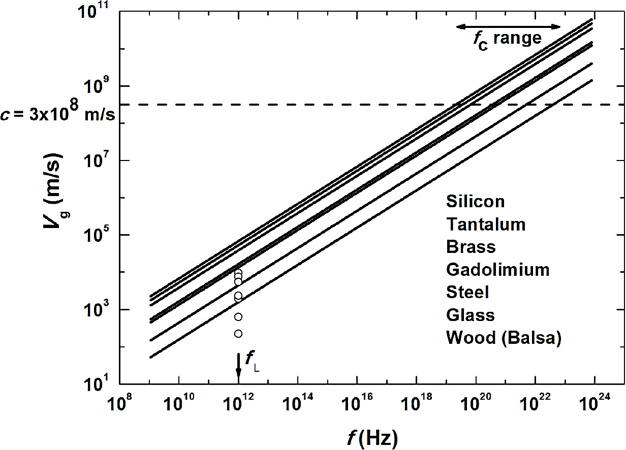
Figure 1 Group velocity as a function of frequency for the materials shown in Table I. The critical frequency range is shown with the horizontal arrow. The speed of light in vacuum is shown with the horizontal line. Values of the second sound velocity for each material are shown with open circles in the figure. Note from Eqs. (10) and (14) that they are related to the group velocity value evaluated at the frequency f = fL =1/τ, namely υg (fL ), by u = υg (fL )/(4π1/2) ∼ υg (fL )/7.
Thus, several questions remain open in TWs physics: What is the TWs behavior at frequencies in the vicinity of fL? At which frequency does the TWs velocity actually change from Vp to u, thus becoming independent on modulation? Although part of this topic has been discussed before 3-5, the debate is not settled, and new experiments and theoretical analysis are needed to understand it better and to shine light on some open questions in the analysis of heat transfer phenomena, in particular those taking place in the presence of periodical heat sources, and to motivate further analysis and discussion on this topic not only between students and teachers, but also among researchers dealing with heat propagation problems under time varying periodical heating conditions. In the past, hyperbolic non-Fourier conduction has strictly been studied from a mathematical viewpoint with insufficient attention to its practical importance. Non-Fourier effects have long been known to exist in the form of second-sound thermal waves in superfluid helium 7. More recently, they have been observed in a variety of phenomena involving ultrafast heating such as supernovae explosions 14, ultrafast laser heating 15 and complex fluids (e.g. colloidal suspensions of nanometer sized particles in basic fluids, where heat transfer times can be substantially reduced due to the reduced dimensions pf the particles) 16-17. Therefore, the existence of non-Fourier heat transfer is a topic of importance to be introduced in modern physics courses. Finally, it is worth mentioning that the hyperbolic heat diffusion equation is one of the possible solutions to avoid the inconsistence of the parabolic approach, which violates the special relativity theory at very high modulation frequencies. However, some authors 16 suggest that the hyperbolic approach also violates the second law of thermodynamics in the very high modulation frequency regime, since heat can flow from the colder region to the hotter in the sample, against the temperature gradient. It is sure that this subject is not closed yet!

