


 nueva página del texto (beta)
 Inglés (pdf)
 Artículo en XML
 Referencias del artículo
 Enviar artículo por email
 Citado por SciELO
  Similares en
SciELO
Similares en
SciELO 
 Permalink
Introduction
Among the life-history evolution models, bet-hedging has been proposed as a good explanatory model for those species with low survivorship in early stages, inhabiting seasonally variable environments, and have reduced reproductive effort (Charnov, 2002, 2005; Enium & Fleming, 2004). Life-history evolution is closely linked with the environmental factors met by the organisms during speciation or local adaptation (Roff, 2002; Stearns, 1992), then, the reproductive output will correlate with environmental conditions by moving forward (reduced reproductive output) or reverse (increment in output) to a bet-hedging life history strategy under high or less environmental (i.e., climate) variability, which represents a direct effect of the environment on the fitness of local populations (Breandle et al., 2011; Roff, 1981, 2002; Stearns, 1989, 1992).
Reproductive output components such as clutch/litter size, egg/neonate size, clutch/litter frequency, and reproductive effort (relative clutch/litter mass) can show plasticity (Shine & Brown, 2008; Shine & Schwarzkof, 1992; Smith & Fretwell, 1974; Tinkle, 1969; Tinkle & Hadley, 1975; Tinkle et al., 1970; Vitt & Prince, 1982). Thereof, plasticity responses in life history traits may also occur among populations or lineages according to the environmental factors they faced during its lifetime (Macip-Ríos et al., 2017; Shine & Schwazkopf, 1992), especially if the environment changes rapidly or if it is seasonally variable, with a higher degree of stochasticity. Hence it is important to investigate the life-history variation during climate change to asses population viability of lineages with potentially imperiled lizards (Sinervo et al., 2010).
In lizards and snakes several life history traits could be fixed or be highly variable (Tinkle et al., 1970). The evolution of life-history traits such as body size, reproductive effort, egg/neonate size, and clutch/litter size could be constrained by the reproductive mode (Rodríguez-Romero et al., 2002; Zúñiga-Vega et al., 2016). Understanding how life-history traits evolve and how they are directly related with environmental variables (i.e., climate, food, light, etc.) is crucial to assess how global environmental changes may affect species occurrence in a fast-changing world (Angilletta et al., 2004; Brandt & Navas, 2011).
There is extensive evidence that lizards have the capacity to adapt to variable environmental conditions (Angilletta et al., 2004; Chamaillé-Jammes et al., 2006; Huey et al., 2012; Logan et al., 2014). That is why it is so important to analyze possible complex interactions between life-history traits such as reproductive mode and body size with reproductive output and with historical environmental (climatic) variables (Andrews & Schwarzkopf, 2012; Meiri et al., 2013).
We used as a study system the spiny lizards from the genus Sceloporus (Iguanidae: Phrynosomatidae). These lizards have been recognized as a suitable model because they inhabit several types of environments within an elevation range from sea level to near 4,000 m (Mathies & Andrews, 1995). Spiny or Sceloporine lizards are exclusive from North America and the lineage includes both, oviparous and viviparous species, a trait that evolved at least 6 times in their evolutionary history (Lambert & Wiens, 2013). The lineage is particularly diverse in Mexico and the southwestern US (Flores-Villela & García-Vázquez, 2014). The referred characteristics make this group of lizards an ideal system to test the evolution of the reproductive output and its relationship with climatic variables at a local scale.
Sceloporine lizards are also facing a population decline due to climate change (Sinervo et al., 2010). According to the latest forecasts, the mean temperature would rise 1.5 °C between 2030 and 2052 (IPCC, 2018). This represents a potential threat to biodiversity at the global and local scale (Tewksbury et al., 2008), and particularly for ectotherms such as reptiles. The global climate change will increase the variation in rainfall and climatic stability leading to fast environmental temperature warming and/or atypical dry conditions episodes (Walters et al., 2012). These new environmental conditions will affect lizards (Deutsch et al., 2008; Huey et al., 2012; Scheffers et al., 2013), which are highly sensitive to environmental temperature variation. Most of their basic biological functions (physiological, reproductive, metabolic, and locomotion) occur within a narrow body temperature range (Angilletta, 2009). Frequently, these body temperature ranges could be evolutionarily static (Grigg & Buckley, 2013), which could drive to short-term extinction processes when environmental conditions change rapidly (Sinervo et al., 2010).
The aim of this study was to analyze the potential correlations between reproductive output traits with environmental variables (climate variation) in a lineage of lizards with different reproductive modes. We hypothesize that the reproductive output of viviparous and oviparous species will correlate with environmental conditions by moving forward to a bet-hedging life history strategy (reduced reproductive output) under high climate variability.
Materials and methods
To explore how reproductive output evolved in spiny lizards (Sceloporus), we conducted a comparative study using the reproductive and phylogenetic data available from the genus. We revised the literature for available data on body size (snout-vent length-SVL), clutch/litter size (CS/LS), and reproductive effort (relative clutch mass or litter) (RCM/RLM, Cuellar, 1984); we also added unpublished data (Table 1). We revised Leaché (2010), Wiens and Reeder (1997), and Wiens et al. (2010), for a phylogenetic hypothesis that better fit our reproductive output database and to have at least one representative taxa from the entire Sceloporine lineage within the phylogeny. In other words, we tried to match the OTU’s present in each topology with the reproductive output data base we gathered.
Table 1 Life-history traits evaluated among the Sceloporus phylogeny. O = Oviparous, V = viviparous. RMC = Reproductive clutch mass, RLM = reproductive litter mass, CS = clutch size, LS = litter size, SVL = snout-vent length (body size).
| Species | Rep. Mode | RCM/ RLM | CS/ LS | SVL | Body mass | Locality | Source |
| S. ochoterenae | O | 0.147 | 5 | 46.4 | 3.34 | Cerro calera chica, Morelos, Mexico | Bustos-Zagal et al., 2011 |
| S. jalapae | O | 0.47 | 5.6 | 46 | Tehuacán, Puebla, Mexico | Ramírez-Bautista et al., 2005 | |
| S. gadoviae | O | 0.6 | 3.9 | 50.4 | 6.03 | Tehuacán, Puebla, Mexico | Ramírez-Bautista et al., 2005 |
| S. melanorhinus | O | 0.65 | 7.7 | 87.9 | Chamela, Jalisco, Mexico | Ramírez-Bautista et al., 2006 | |
| S. torquatus | V | 0.3 | 6.5 | 90.6 | 26.17 | Pedregal de San Ángel, México D.F. | Feria-Ortiz et al., 2001 |
| S. jarrovi | V | 0.468 | 4.9 | 60.9 | 14.57 | Pinal de Amoles, Querétaro, Mexico | Ramírez-Bautista et al., 2002 |
| S. microlepidotus | V | 0.48 | 5.2 | 48.5 | Zoquiapan Edo. de Méx., Mexico | Guillette & Casas-Andreu, 1980 | |
| S. duguessi | V | 0.192 | 4.6 | 61.5 | Tzintzuntzan, Michoacán, Mexico | Ramírez-Bautista y Dávila, 2009 | |
| S. poinsetti | V | 0.5 | 6.3 | 85.8 | 30.94 | Mapimí, Durango, Mexico | Gadsen et al., 2005 |
| S. cyanogenys | V | 0.3 | 13 | 106 | 39 | Webb, County Texas, USA | Hunsaker, 1959; Garrick, 1974 |
| S. serrifer | V | 0.0548 | 3.9 | 82.2 | 23.47 | Conkal, Yucatán, Mexico | López-Alcaide, unpublished data |
| S. mucronatus | V | 0.27 | 5.1 | 83.5 | 19.47 | Zoquiapan, Edo. de Méx., Mexico | Rodríguez-Romero et al., 2005 |
| S. macdougalli | V | 0.116 | 3.7 | 74.8 | 16.03 | Santa Cruz Bamba, Oaxaca, Mexico | López-Alcaide, unpublished data |
| S. mucronatus aureolus | V | 0.0842 | 6.5 | 71.9 | 16.27 | Tlaxiaco, Oaxaca, Mexico | López-Alcaide, unpublished data |
| S. grammicus | V | 0.49 | 5.1 | 50.9 | 5.18 | Pachuca, Hidalgo, Mexico | Ramírez-Bautista et al., 2009 |
| S. formosus | V | 0.433 | 6.6 | 64.8 | 12.62 | San Pablo Etla, Oaxaca, Mexico | Ramírez-Bautista y Pavón, 2009 |
| S. horridus | O | 0.7 | 15 | 91.4 | 19.46 | El Rodeo, Morelos, Mexico | Valdéz-González & Ramírez-Bautista, 2002 |
| S. spinosus | O | 0.75 | 19 | 98.6 | Las Minas, Puebla, Mexico | Valdéz-González & Ramírez-Bautista, 2002 | |
| S. undulatus | O | 0.43 | 9.1 | 71.9 | 9.51 | Burlington, New Jersey, USA | Angilletta et al., 2001 |
| S. virgatus | O | 0.289 | 10 | 61.5 | 8.48 | Chiricahua, Arizona, USA | Smith et al., 1995 |
| S. occidentallis | O | 0.318 | 4.2 | 74.4 | 14.29 | Lyle, Washington, USA | Sinervo et al., 1991 |
| S. scalaris | O | 0.86 | 9.4 | 52.8 | 5.8 | Cochise, Arizona USA | Mathies & Andrews, 1995 |
| S. aeneus | O | 0.24 | 3.9 | 47.5 | 4.3 | Milpa Alta, D.F., Mexico | Rodriguez-Romero et al., 2002 |
| S. bicanthalis | V | 0.52 | 5.9 | 49.2 | 4.18 | Zoquiapan, Edo. de Méx. Mexico | Rodriguez-Romero et al., 2002 |
| S. orcutti | O | 0.6 | 11 | 92 | 22.63 | Riverside, California, USA | Mayhew, 1963 |
| S. graciosus | O | 0.196 | 3.7 | 56.4 | 6.8 | National Park Zion, Utah, USA | Tinkle et al., 1993 |
| S. variabilis | O | 0.212 | 4.6 | 55.4 | 7.19 | Bastonal, Veracruz, Mexico | Benabib, 1994 |
| S. utiformis | O | 0.6 | 6.9 | 63.8 | 9.18 | Chamela, Jalisco, Mexico | Ramírez-Bautista & Gutiérrez-Mayén, 2003 |
| S. pyrocephalus | O | 0.78 | 5.8 | 47 | Tejupilco, Edo. de Méx. Mexico | Ramírez-Bautista & Olvera-Becerril, 2004 | |
| S. bicanthalis_2 | V | 0.47 | 7.2 | 52.1 | 5.97 | Nevado de Toluca, Edo. de Méx., Mexico | Rodríguez-Romero et al., 2004 |
| S. jarrovi_2 | V | 0.468 | 7.8 | 72.9 | Pabellón de Arteaga, Aguscalientes, Mexico | Ramírez-Bautista et al., 2002 | |
| S. mucronatus_2 | V | 0.37 | 6.5 | 79.4 | 19.47 | Tecocomulco, Hidalgo, Mexico | Villagrán et al., 2009 |
| S. torquatus_2 | V | 0.34 | 9.7 | 72 | 26.17 | San Juan Teotihuacán, Edo. de Méx. Mexico | Guillette & Méndez-de La Cruz, 1993 |
| S. horridus_2 | O | 0.0251 | 16 | 94 | 24.49 | Xalitla, Guerrero, Mexico | López-Alcaide unpublished data |
| S. occidentallis_2 | O | 0.281 | 3.9 | 74.4 | 14.29 | Terrebone, Oregon, USA | Sinervo et al., 1991 |
| S. undulatus garmani | O | 1 | 6.2 | 64.6 | 5.26 | Statfford, Kansas, USA | Ferguson & Snell, 1986 |
| S. variabilis_2 | O | 0.203 | 4.3 | 55.4 | 7.04 | Montepío, Veracruz, Mexico | Benabib, 1994 |
| S. spinosus albiventris | O | 0.0503 | 10 | 74 | 15 | Chamela, Jalisco, Mexico | López-Alcaide unpublished data |
Since we did not gather data for all the species included in the consulted phylogenies (Wiens & Reeder, 1997; Wiens et al., 2010), we decided to generate our own phylogeny that matched our database. We downloaded the sequences used by Leaché (2010) from GenBank (Geer et al., 2010) for the nuclear markers: RAG-1, BDNF, RNA finger print protein 35, and the PNIN gene. We also used the available mtDNA sequences for 12S, NAD1, and NAD4. Sequence alignment was performed using Clustal W (Larkin et al., 2007). The nucleotide data base was run in Modeltest 3.06 (Posada, 2008; Posada & Crandall, 1998) to determine the evolution model used in the phylogenetic inference, then based on Leaché (2010) topology we constructed a template to perform a constrained phylogenetic analysis to conserve Leaché (2010) main topology but setting free the branch calculation for the new topology. We performed a maximum likelihood phylogenetic analysis using RAxLM (Stamatakis, 2014) in a graphical interface called raxmlGUI (Silvestro & Michalak, 2011). Uta stansburiana was used as out-group. We performed 1,000 random bootstrap re-samples to calculate branch support. The phylogenetic tree was visualized and edited in Figtree 1.4.2 (http://tree.bio.ed.ac.uk/software/figtree/).
We used WorlClim data layers to calculate climatic variation per locality (or localities) from where life-history data were originally sampled (Hijmans et al., 2005). To extract climate data, we used a 100 × 100 m2 grid to extract average climatic data. To compare temporal variation between localities, we searched for 2 basic types of climatic variables; temperature, including mean, minimum, and maximum monthly temperature; and precipitation, including total rain per month, monthly mean evapotranspiration, and maximum rain per day. Since our objective was to describe temporal environmental variation as a main assumption for the bet-hedging life-history strategy (Charnov, 2002, 2005), we calculated standard deviations for each variable and a mean of standard deviations for every type of variable, thermal (TV) and rain variation (RV). We also combined both standard deviations of variables in an average of thermal and rain variation, which was called total climate variation (TCV).
The dataset was analyzed in 2 basic ways: 1) by standard parametric statistical analyses, and 2) by comparative phylogenetic methods (Goolsby, 2015). To determine the correlation between body sizes with reproductive output, we conducted a series of linear correlations. We compared life-history traits of oviparous with viviparous species by an Ancova, using the body size as a covariate (Zar, 1999). This procedure did not imply a phylogenetic correction.
Since our data set is hierarchically ordered following the phylogenetic relationships, we proceeded using phylogenetic comparative methods (Harvey & Pagel, 1991). We used Felsenstein phylogenetic independent contrast (PIC) to identify correlations between life-history traits (Felsenstein, 1985, 2008). We ran the PIC tests with Mesquite ver. 3.04 (Maddison & Maddison, 2018) using the PDAP package (Garland et al., 1999; Garland & Ives, 2000).
A phylogenetic Anova was also used to compare between oviparous and viviparous species (Garland et al., 1993). We ran the phylogenetic Anova in phytools in R (R Development Core Team, 2008; Revell, 2012). To detect the phylogenetic signal on the reproductive output traits evaluated, we used the K statistic also in phytools (Bloomberg et al., 2003; Revell, 2012). K statistic works as a gauge of phylogenetic signal in a trait that allows the comparison between traits and between trees (Münkemüller et al., 2012). Transformations, parametric assumptions tests, and standard statistical analyses were conducted with JMP ver. 5.0.1 (SAS Institute, 2002).
Results
Data set was composed by 38 operative taxonomic units (OTU’s), including 28 species, approximately 31% of all the species contained in the lineage (Table 1). Some species were over represented by more than 1 population, we included all observations to achieve a larger sample. We gathered information from 21 oviparous and 17 viviparous species. Our sampling allowed to include at least 1 species of each of the major and minor clades of the lineage. The data set comprised a 27° range in latitude from Sceloporus occidentalis from Oregon (44.32° N), to Sceloporus mucronatus from Oaxaca (17.26° N), Mexico. Overall, according to our database and among the Sceloporus lineage, body size (SVL) averages 70 mm (± 16.8, range 106-46), body mass 14.28 g (± 9.04, ranges 3.34-39), clutch size or litter size 7.2 (± 3.6, range 4-19), and relative clutch mass or relative litter mass 0.38 (± 0.21, ranges 86-0.025).
When we compared oviparous with viviparous taxa in a phylogenetic context (Fig. 1), the phylogenetic Anova did not detect significant variation in body size (F = 0.25, p = 0.808), CS/LS (F = 0.36, p = 0.74), and RCM/RLM (F = 0.007, p = 0.95), nevertheless, the phylogenetic signal was statistically detectable for body size (K = 1.11, p = 0.001), body mass (K = 1.42, p = 0.001), and CS/LS (K = 0.6, p = 0.047), but not for RCM/RLM (K = 0.18, p = 0.99).
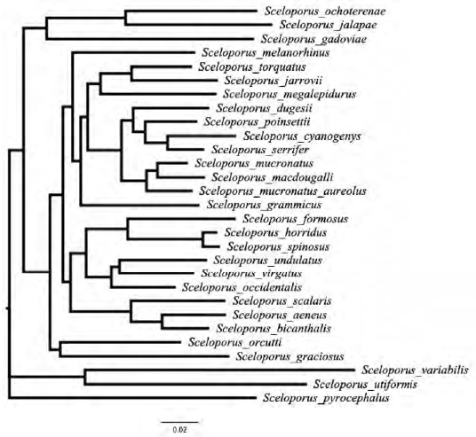
Figure 1 Phylogenetic tree used for comparative phylogenetic methods. Outgroup was removed from the analysis.
Felsenstein independent contrast analysis between climatic variables and life-history traits showed a significant inverse correlation between minimum environmental temperature (T°min) and average environmental temperature (T° env ) with CS/LS (r2 = -0.43, F = 7.41, p = 0.01 and r2 = -0.33, F = 4.40, p = 0.04; Table 2). Also, body size and body mass showed direct correlations with CS/SL (r2 = 0.56, F = 16.87, p = 0.00021 and r2 = 0.45, F = 7.61, p = 0.009). No correlations between other life history traits or/with environmental variables were detected (Table 2).
Table 2 Correlations through the origin after phylogenetic independent contrast between life-history traits and climatic variables for the Sceloporine sample. RMC = relative clutch mass, RLM = relative litter mass, CS = clutch size, LS = litter size, body size = snout vent length, T°max = maximum monthly temperature at site, T°min = minimum monthly temperature at site, T°env = mean monthly temperature, Prec(X) = monthly precipitation, SD = standard deviation.
| Y | X | r2 | F | p | Origin | Slope |
| CS/BS | Body size | 0.56 | 16.87 | 0.00021 | 0.49 | 0.13 |
| RCM/RLM | Body size | 0.21 | 1.71 | 0.19 | -3.07 | 4.78 |
| CS/BS | Body mass | 0.45 | 7.61 | 0.009 | 1.26 | -0.02 |
| RCM/RLM | Body mass | -0.08 | 0.23 | 0.06 | -0.09 | -0.31 |
| CS/BS | T°max | -0.21 | 1.68 | 0.20 | 0.41 | -0.50 |
| RCM/RLM | T°max | -0.16 | 0.09 | 0.32 | 0.53 | -1.07 |
| Body size | T°max | -0.01 | 0.005 | 0.94 | 0.22 | -0.12 |
| Body mass | T°max | -0.07 | 0.15 | 0.69 | 0.80 | -0.15 |
| CS/BS | T°min | -0.43 | 7.41 | 0.01 | -0.29 | 0.52 |
| RCM/RLM | T°min | -026 | 2.42 | 0.12 | 0.75 | -0.77 |
| Body size | T°min | -0.04 | 0.06 | 0.80 | 0.11 | -0.03 |
| Body mass | T°min | -0.11 | 0.30 | 0.58 | 1.67 | -0.18 |
| CS/BS | T°env | -0.33 | 4.40 | 0.04 | 0.45 | -0.54 |
| RCM/RLM | T°env | -0.25 | 2.50 | 0.12 | 1.00 | -1.40 |
| Body size | T°env | -0.13 | 0.61 | 0.43 | 0.34 | -0.20 |
| Body mass | T°env | -0.17 | 0.90 | 0.34 | 0.23 | -0.15 |
| CS/BS | Prec (X) | -0.02 | 0.02 | 0.87 | 0.11 | -0.01 |
| RCM/RLM | Prec (X) | 0.05 | 0.09 | 0.76 | 0.39 | 0.004 |
| Body size | Prec (X) | -0.04 | 0.07 | 0.78 | 0.35 | -0.03 |
| Body mass | Prec (X) | -0.08 | 0.20 | 0.65 | 5.03 | -0.44 |
Table 3 Correlations between the life-history traits and environmental variables analyzed for the Sceloporine lineage. RMC = Relative clutch mass, RLM = relative litter mass, CS = clutch size, LS = litter size, body size = snout vent length, T°max = maximum monthly temperature at site, T°min = minimum monthly temperature at site, T°env = mean monthly temperature, Prec(X) = monthly precipitation, SD = standard deviation.
| Y | X | r2 | F | p | Origin | Slope |
| CS/BS | Body size | 0.29 | 14.88 | 0.005 | -2.12 | 0.95 |
| RCM/RLM | Body size | 0.03 | 1.2 | 0.28 | 1.32 | -0.59 |
| CS/BS | Body mass | 0.15 | 5.26 | 0.02 | 1.24 | 0.24 |
| RCM/RLM | Body mass | 0.044 | 1.31 | 0.26 | -0.64 | -0.24 |
| CS/BS | T°max | 0.01 | 0.45 | 0.50 | 1.20 | 0.18 |
| RCM/RLM | T°max | 0.005 | 0.21 | 0.64 | -0.34 | -0.24 |
| Body size | T°max | 0.03 | 1.31 | 0.25 | 3.61 | 0.17 |
| CS/BS | T°min | 0.002 | 0.07 | 0.78 | 1.95 | -0.03 |
| RCM/RLM | T°min | 0.071 | -0.28 | 0.37 | -0.28 | -0.37 |
| Body size | T°min | 0.022 | 0.71 | 0.40 | 4.0 | 0.06 |
| CS/BS | T°env | 0.006 | 0.22 | 0.63 | 1.55 | 0.10 |
| RCM/RLM | T°env | 0.04 | 1.76 | 0.19 | 0.44 | -0.54 |
| Body size | T°env | 0.004 | 0.14 | 0.70 | 4.06 | 0.04 |
| CS/BS | Prec (X) | 0.006 | 0.23 | 0.62 | 1.80 | 0.02 |
| RCM/RLM | Prec (X) | 0.06 | 2.59 | 0.11 | -1.56 | 0.12 |
| Body size | Prec (X) | 0.003 | 0.12 | 0.72 | 4.17 | 0.008 |
| CS/BS | SD of T°max | 0.0001 | 0.0048 | 0.94 | 1.86 | 0.007 |
| RCM/RLM | SD of T°max | 0.0002 | 0.009 | 0.922 | -1.17 | 0.02 |
| Body size | SD of T°max | 0.00006 | 0.002 | 0.96 | 4.20 | -0.003 |
| CS/BS | SD of T°min | 0.01 | 0.37 | 0.54 | 1.83 | 0.062 |
| RCM/RLM | SD of T°min | 0.013 | 0.50 | 0.48 | -1.23 | 0.13 |
| Body size | SD of T°min | 0.05 | 2.23 | 0.14 | 4.15 | 0.08 |
| CS/BS | SD of T°env | 0.0008 | 0.03 | 0.86 | 1.86 | 0.01 |
| RCM/RLM | SD of T°env | 0.0007 | 0.028 | 0.86 | -1.17 | 0.03 |
| Body size | SD of T°env | 0.01 | 0.58 | 0.44 | 4.17 | 0.04 |
| CS/BS | SD of Prec (X) | 0.01 | 0.40 | 0.53 | 1.80 | 0.024 |
| RCM/RLM | SD of Prec (X) | 0.04 | 1.82 | 0.18 | -1.42 | 0.09 |
| Body size | SD of Prec (X) | 0.02 | 1.00 | 0.32 | 4.14 | 0.02 |
Standard statistical analyses only showed moderate to weak correlations between body size (SVL), CS/LS (r2 = 0.29, p = 0.005) and body mass to CS/LS (r2 = 0.15, p = 0.02). No other correlations were detected, not even with any of the environmental variables (Table 3). We found significant variation in body mass between oviparous and viviparous species (t = 2.49, p = 0.02), but we did not find any variation in body size (t = 0.74, p = 0.46). We ran an Ancova using body mass as a covariable to compare CS/LS and RCM/RLM. Variation was only detected for CS/LS (F = 7.75, p = 0.002) among reproductive mode. According to our results oviparous species produce larger clutches than viviparous ones. Reproductive effort (RCM/RLM) did not show any variation (F = 0.32, p = 0.72) between reproductive mode.
Discussion
As expected, and described in single species studies (e.g., Abell, 1999; Benabib, 1994; Feria et al., 2001; Gadsden et al., 2005; Mathies & Andrews, 1995), clutch/litter size was positively correlated with body size. Longer females produce larger clutches or litters, which under certain environmental conditions is advantageous to increase fitness (Roff, 2002; Stearns, 1992). According to our results, at lower environmental temperatures, females tend to produce smaller clutches/litters, which seem to be a direct response to a critical thermal environment. We did not test the correlation of hatchling size with environmental variables, but the clutch/litter size correlation with body size suggests a trade-off resolution through few, but large offspring in cooler habitats. This response seems logical to provide offspring with more mass and energy in colder environments, however the production of more offspring (with smaller size) in tropical environments (also more thermally stable) could be selected (Mesquita, Costa et al., 2016; Mesquita, Gomes-Faria et al., 2016). Our interpretation agrees with Bergmann’s Rule, which has been tested with several groups of vertebrates such as mammals (Ashton et al., 2000), turtles (Lewis et al., 2018), lizards, and snakes (Angilletta et al., 2004; Ashton & Feldman, 2003).
Our analysis showed that oviparous and viviparous species have equal CS/LS and reproductive effort when the effect of body size is removed, this result agrees with the correlation of body size with CS/LS and indicates that body size has a deep influence in CS/LS and then in life history variation, which also agrees with Mesquita, Costa et al. (2016) who did not find differences in CS/LS among several lineages of lizards with different reproductive mode. Oviparous and viviparous species did not differ in their reproductive output, nevertheless, both reproductive modes have been hypothesized as adaptations to thermal conditions (cold weather hypothesis; Lawing et al., 2016; Martínez-Méndez et al., 2019; Shine, 2004) rather than reproductive output strategies. Results from Zúñiga-Vega et al. (2016) support that the correlation between life history traits with environmental factors in prhynosomoatid lizards, could be related to their evolutionary history under cooling conditions.
Bloomberg et al. (2003) mentioned that the K statistic for the phylogenetic signal could show high values for large sample sizes when concerning body size or body mass. We obtained higher values for both traits. Then, according to this interpretation, reproductive output could potentially be affected by the phylogenetic inertia of body size and its correlation with other reproductive output traits, however, reproductive effort seems not to be affected by the phylogenetic signal, body size or any of the environmental variables tested. It was interesting to discover a correlation of reproductive effort with climatic variation. This also has been reporterd for other groups of lizards (Mesquita, Costa et al., 2016), snakes (Shine & Schwarzkopf, 1992), and turtles (Macip-Ríos et al., 2017). Recently, Mesquita, Gomes-Faria et al. (2016) argued that lizard life history strategies could be classified by clutch size, the age of maturity, and investment per progeny (reproductive effort). Based on these 3 axes, lizards occupy a narrow space in a 3D plot, going from low clutch size, low age at maturity, and middle investment per progeny, to low clutch size, delayed age at maturity, and low reproductive effort. It seems that Sceloporine lizards fit the general pattern. However, our lack of data of several life-history traits to compare with Mesquita, Gomes-Faria et al. (2016) data limits the overall interpretation.
Our results agree with Mesquita, Costa et al. (2016) main conclusions of high phylogenetic signal in RCM/RLM, CS/LS, and body size and correlation between climatic variables with life-history traits. It seems that deep evolutionary history has an important role in life-history variation. Compared with Mesquita, Costa et al. (2016) and other studies of life-history patterns in lizards (Dunham et al., 1988; Mesquita, 2010; Miles & Dunham, 1992; Vitt & Congdon, 1978; Zúñiga-Vega et al., 2016), our results match in a general way what has been described as lizard life history strategy, however it is interesting how the reproductive mode in the life-history traits mentioned above has no influence (except CS/LS). Recently Zúñiga-Vega et al. (2016) also documented the same lack of influence of reproductive mode and suggested how viviparity could constraint the evolution of life-history traits, rather than oviparity. Because our main objective was to test the bet-hedging strategy, we consider that Sceloporus lizards partially followed the bet-hedging predictions, nevertheless, other life-history models should be tested in Sceloporine lizards such as the fast-slow continuum hypothesis as pointed out by Pérez-Mendoza and Zúñiga-Vega (2014).
Since climate change will affect thermal niches, lizard life-history could face severe constraints that could reduce species geographic distributions and the viability of local populations (Gadsden et al., 2018; Martínez-Méndez et al., 2019). Lawing et al. (2016) demonstrated that Sceloporine lizards diversified during the last ice age, and viviparity became an important trait to colonize new environments, therefore during global warming and generalized climate change, the perspectives of survivorship of this group of lizards could be imperiled. Sinervo et al. (2010) demonstrated important population exctinctions on the genus Sceloporus by climate change due to a direct consequence of the restrictions that high environmental temperatures impoose on their activity out of shelters, which reduces their food intake and their reproductive cycles. Moreover, Sceloporine lizards exhibit a conserved physiology relative to reproductive traits (high phylogenetic signal). A good example of this is the narrow temperature range of healthy embryo development, which occurs between 31.3 ± 0.2 and 32.8 ± 0.1 °C (Andrews et al., 1997). In addition, it is also known that most reptiles have limited dispersal abilities and Sceloporine lizards are not the exception. To face a fast-climatic change, spiny lizards may not be able to migrate in the short term to sites with suitable conditions. Consequently, these lizards are among the most vulnerable groups of organisms threatened by climatic change (Araujo et al., 2006; Carvalho et al., 2010; Chen et al., 2011).
Nevertheless, lizards are not inert biological entities unable to respond to environmental variation, it would be reasonable to expect that they may show some type of adjustment of life history traits to thermal conditions when climate changes occur. Environmental temperatures can exert strong selection pressures and some species may exhibit rapid adaptation, either genetically regulated or by phenotypic plasticity (Moritz et al., 2012). Hence, a thermal regime that spiny lizards could experiment could drive changes in their life history traits (if there is enough heritability; Bradshaw & Holzapfel, 2006; Kellermann et al., 2012) and confer resiliency to warmer thermal conditions in a relatively short period of time, and then favor populations to increase their survival probabilities or face local extinctions (Leal & Gunderson, 2012; Logan et al., 2014; Sinervo et al., 2010).

