


 nueva página del texto (beta)
 Inglés (pdf)
 Artículo en XML
 Referencias del artículo
 Enviar artículo por email
 Citado por SciELO
  Similares en
SciELO
Similares en
SciELO 
 Permalink
Introduction
The degradation of natural systems caused by human activities is one of the main factors that increase land- cover change and biodiversity loss (Bertzky et al., 2012; Lambin et al., 2003). Anthropogenic activities have led to an approximately 50% reduction in global land-cover (DeFries, 2008). This loss is concentrated primarily in developing tropical countries with gentle slopes, where livestock development and agricultural production are high (Lambin et al., 2003; Lugo, 1988; McDonald et al., 2007). Tropical forest ecosystems contain almost 70% of the world’s biodiversity and are the most affected ecosystems by land-cover change (Lambin et al., 2003; Pau et al., 2011). Given this scenario, governments around the world have taken different approaches to reduce the loss of ecosystems, such as the creation of protected areas (PAs) or priority regions (PTRs) for conservation (Beresford et al., 2011; Bertzky et al., 2012). PAs are spaces for biodiversity conservation, and they attempt to maintain the integrity of ecosystems and environmental services and are supported by laws that regulate anthropogenic activities (Ferreira et al., 2013; IUCN, 2005). However, inside various PAs and PTRs, some degree of deterioration continues (Joppa & Pfaff, 2011; Leisher et al., 2013; Mascia & Pailler, 2011; McDonald et al., 2007; Nagendra, 2008; Sánchez-Colón et al., 2009).
Loss of vegetal coverage inside PA can result from activities that occur inside and on their peripheries (DeFries, 2008). The loss of coverage that occurs on the peripheries can lead to isolation from other PAs that consequently reduces the genetic flow between populations (IUCN, 2005; Mas, 2005b; Hansen & DeFries, 2007). Natural resources to incorporate new PAs are limited; therefore, we need to select the most feasible areas for conservation with high diversity that contain distinctive biota, where we can propose specific conservation strategies for each area. The peripheries of a PA play an important role in the conservation of natural resources because they contain high diversity (IUCN, 2005) and are known as priority regions (PTRs) for conservation (Bertzky et al., 2012). In 2005, 11,581 PTRs were reported worldwide, and only 30% were completely or partially within a PA (Ricketts et al., 2005). Most of the PTRs do not have any legislation to protect them, driving them to a remarkable risk by deterioration (Bertzky et al., 2012). Therefore, it is necessary to estimate the trends of past changes, as well as the types of coverages most affected, in order to identify areas with the greatest risks from land-cover change and to propose conservation strategies.
The objective of PA and PTR is to preserve as many species as possible. Consequently, these ought to include areas that increase the diversity and environments that differ from those already protected (Halffter, 2011). These conditions are necessary for gastropods, aquatic plants and pteridophytes, which require different aquatic conditions to survive (Venegas-Barrera et al., 2015). Gastropods have a greater affinity for humid environments and elevated temperatures, such as in tropical rain forests (Correa-Sandoval et al., 2009). Pteridophytes also require humid environments and available water for the development of spores; once established they can tolerate different environments. Finally, aquatic plants require permanent water bodies or, at least, damp soil to develop properly (Sculthorpe, 1985). These organisms depend on water to develop (Mora-Olivo et al., 2008) because they are sensitive to changes in land conditions. Therefore, it is necessary to associate land-cover changes with the richness maps of these organisms to select the most feasible areas for their conservation.
Mexico is a megadiverse country because it contains approximately 12% of the planet’s biodiversity (Torres, 2004). In addition to this, Mexico has one of the highest deforestation rates in the world. The country loses approximately 523,639 ha/year, of pristine forest and the forests located in the coastal plains are the most affected (Challenger et al., 2009; Flores & Gerez, 1994). Since the late seventies, until the 21st century, 181 PAs have been declared, and each one has ecological characteristics relevant to conservation (Bertzky et al., 2012; Le Saout et al., 2013). However, in 35 of 81 PAs, loss of native vegetation continued (Figueroa & Sánchez-Cordero, 2008), even though there is legislation that regulates the activities within the area. Furthermore, in 2007, the Comisión Nacional para el Conocimiento y Uso de la Diversidad and other institutions (Conanp, TNC and Pronatura), proposed areas that allow the different elements of biodiversity to accomplish their conservation targets in the smallest area, which was named terrestrial priority sites (PTSs). PTSs recognize 3 categories of priority in function of endemism, risk of extinction, rarity of species, as well as critical vegetation types, richness and land- cover change. The PTRs and PTSs that are located either partially or completely within the periphery of a PA are at a greater risk because they do not have any legislation to protect their ecosystems or their functional ecological integrity from anthropogenic activities. In addition, PTSs proposal were generated with vertebrates and plant reported in NOM-059, excluding invertebrates and other plant species. Therefore, it is necessary to identify more susceptible PTRs and PTSs for conservation due to change of vegetation cover.
The state of Tamaulipas is a priority area for estimating the changes in land-cover because it is one of the most diverse states in the northeastern region of Mexico (Treviño-Carreón & Valiente-Banuet, 2005). Tamaulipas also has the highest deforestation rates in Mexico, with an annual loss of 52,000 ha of vegetal cover (Aguilar et al., 2000). The most affected environments include rainforests and xeric scrublands, which are mostly located in areas with low slopes and foothills (Cotler, 2010). The state has designated 9 local PAs, 2 federal PAs, and 12 PTRs, all of which are mostly situated in mountain areas (Arriaga et al., 2000). While the state has decreed many PAs and PTRs, several areas with high species richness that could be affected by land-cover changes are still unidentified. The 38.7% of Tamaulipas surface is classified in one of the 3 categories of priorities, where extreme and high priority categories concentrate the 23.7% surface. Therefore, in this study we identify spatial patterns of richness, areas with distinctive biota (strict, subaquatic, and tolerant aquatic herb species, ferns, and gastropods) and their associations with land-cover changes that occurred between 1986- 2002 and 2002-2011 in 2 Aps, 5, PTR, and 128 PTSs on Tamaulipas. As well, we identify socioeconomic or environmental conditions that may increase the risk of loss of coverage that increase. The study proposes that a higher richness of aquatic plants, gastropods, and pteridophytes occurs in lowland tropical forests than on the peripheries of a PTR, where the land-cover loss occurs more frequently.
Materials and methods
Land-cover change was calculated 2 PAs (Sierra de Tamaulipas and El Cielo), 5 PTRs (Sierra de San Carlos, Puerto Purificación, San Antonio Peña Nevada, Valle de Jaumave, and Cenotes de Aldama) and 128 PTSs of Tamaulipas, Mexico, which are in the south-central area of the state (Fig. 1a, b). In this area, there is a high concentration of endemic species, and it is a biological diversity hotspot because many tropical species reach their boreal distribution limit in this region (Correa-Sandoval & Rodríguez-Castro, 2005; Mora-Olivo & Villaseñor, 2007; Mora-Olivo et al., 2013; Treviño-Carreón & Valiente- Banuet, 2005). Scrubland and low tropical forests dominate the lower altitudes and coniferous forests, oak and cloud forests dominate the higher altitudes (Treviño-Carreón & Valiente-Banuet, 2005).

We created a 10 km buffer zone from the geographical boundary of each PA and PTR (Arriaga et al., 2000). The polygons were obtained from the digital map collection of the Comisión Nacional para el Conocimiento y Uso de la Biodiversidad (Conabio, http://www.conabio.gob.mx/informacion/gis/). We analyzed the changes inside and outside of conservation areas separately to determinate if the changes were equally frequent in all PAs, PTRs and PTS or if they were concentrated in one (Mas, 2005b). The vegetation layers were obtained from the land-use and vegetation from the Instituto Nacional de Geografía e Informática (INEGI) series I (1986), III (2002a, b) and V (2011) at a spatial scale of 1: 250,000 (http://www.inegi.org.mx/). The land-cover layers have different classifications of vegetation types, so we grouped the vegetation types into native land- cover (mountain cloud forest, temperate forests, scrubland, and tropical lowland forests) and modified land-cover (agricultural and anthropogenic, March-Mifsut & Flamenco-Sandoval, 1996). The land-cover change was calculated between 2 periods, 1986 to 2002 and 2002 to 2011. We estimated changes in vegetation types by intersecting the maps from the 2 periods in PAs, PTRs and PTSs (Fig. 1c, d). The types of changes were categorized into 4 groups: 1) native (N), an area that remained as native land-cover in both periods; 2) modified (M), an area that remained as modified cover in both periods; 3) loss (L), an area that changes from native land-cover to modified cover; 4) gain (G), an area that changes from modified cover to native land-cover.
Deforestation rate (r) was estimated using the equation proposed by the FAO (1996):
where A1 = initial transformed surface, A2 = final transformed surface, and t = years elapsed between t2 and t1 in years.
Additionally, we used types of change to estimate the sequence of land-cover change between 1986-2002 and 2002-2011 in PAs, PTRs, and PTSs, which allows identify the history of change that occurred in the area. We founded 8 types of change: a) native (N), an area that remained as native land-cover from 1986 to 2011; b) gain- native (GN), an area that changes from modified cover to native land-cover (1986-2002) and in 2011 remained as native; c) native-loss (NL), an area that remained as native land-cover from 1986 to 2002 and changes to modified cover in 2011; d) gain-loss (GL), an area that changes from modified cover to native land-cover (1986-2002) and changes to modified cover in 2011; e) loss-gain (LG), an area that changes from native cover to modified land-cover (1986-2002) and changes to native cover in 2011; f) modified-gain (MG), an area that remained as modified land-cover from 1986 to 2002 and changes to native cover in 2011; g) loss-modified (LM), an area that changes from native cover to modified land-cover (1986-2002) and in 2011 remained as modified; h) modified (M), an area that remained as modified land-cover from 1986 to 2011.
Species richness maps were generated from the individual prediction of the geographical distribution of species using the maximum entropy algorithm (ver. 3.2, Phillips et al., 2006). Maximum entropy algorithm is a general-purpose machine learning method with a simple and precise mathematical formulation, and it has several aspects that make it well-suited for species distribution modeling. The collection records for the 5 taxonomic groups of studied species were obtained from 2 databases available online (GBIF [https://www.gbif.org] and Conabio [http://www.conabio.gob.mx/informacion/gis/]; supplemental material) and in published papers (Correa-Sandoval & Rodríguez-Castro, 2005; Correa-Sandoval et al., 2012; Mora-Olivo & Villaseñor, 2007; Mora-Olivo et al., 2008, 2013). The localities that were used include at least their name or the geographical coordinates. If only the names of the localities were reported, then the coordinates were obtained from topographic maps (scale 1: 50,000, INEGI, 2002b) or Google Earth (https://earth.google.com/web/8z). In total, 169 unique localities of gastropods, 714 localities of aquatic plants and 183 localities of pteridophytes were utilized. We only generated potential distribution models for species with at least 7 unique collection localities, which is the minimum number of suggested localities needed to generate distribution maps (Phillips et al., 2006).
The prediction of the geographical distribution was performed using environmental variables representing climate, topography, and vegetation variations. The spatial resolution of the layers was approximately 1 km2 (30 arc seconds). The climatic variables were obtained from WorldClim (www.worldclim.org/), the land-cover variables were obtained from the Global Land-cover Facility (http://www.landcover.org/index.shtml), the aridity index was obtained from (http://csi.cgiar.org/aridity/index.asp) and the topographic variables were obtained from HYDRO1k (http://edc.usgs.gov/products/elevation/gtopo30/hydro/index.html). Terrestrial ecoregions were used to specify extent accessible to the species via dispersal over relevant periods of time (Barve et al., 2011), which reflect the distribution of sharing species and communities that are distinct from those of another ecoregion (Olson et al., 2001). The themed layers were generated with ArcGIS (ver. 10.1 California, ESRI, 2012) and Idrisi Selva (Worcester MA, Clark Lab) software.
The threshold value of the convergence used to find the nearest empirical distribution was 0.00001, with a maximum of 1,000 iterations (Phillips et al., 2004). The model calculated the area under the curve (AUC) to estimate the probability that the generated model was better than a randomly generated model, considering that a perfect rating has an AUC = 1.0. We estimate partial receiver operating characteristic (ROC), which do not require true absences and use total predicted area against false positive rate (http://shiny.conabio.gob.mx:3838/nichetoolb2/). The results are presented as the AUC ratio; when the value moves away from 1.0 the model improves with respect to the random model (Lobo et al., 2007). A presence-absence map of each species was generated by the predictive models using a fixed cumulative value of 10. We generated potential distribution maps for 174 species, where 30 were pteridophytes, 27 gastropods, 30 tolerant aquatic species, 51 subaquatic species, and 36 strict aquatic species. We obtained a richness map by the sum of binary individual species to create maps of species richness for each of the groups.
For each group of species, we identified areas with a distinctive species composition with a generalized k-means analysis. Individual binary maps of geographic distributions were vectorized and intersected to divide the study area into polygons with different composition of species. Polygons were grouped by function of their species composition by a generalized k-means analysis, which finds the optimum partition for dividing several objects into k clusters based in their categorical variables (presence-absence) in Statistica software (StatSoft, 1984). The analysis searches for a combination of sites that maximize significant differences in local species composition among groups based on individual Chi square (X 2) tests for each species. The null hypothesis was that the frequency of sites per group was similar at a probability of 0.05. The result was the assignment of each polygon by a joining table in ArcGIS software (ver 10.0 ESRI).
The richness and species distribution inside and outside of PAs, PTRs, and PTSs. The objective of a protected area is to preserve the highest richness, to contain the primary distribution, and to reduce the rate of land-cover change in each distinctive species area. Therefore, we tested if these ecological variables were higher inside than outside of a PTRs and PTSs for each distinctive species area. We tested if the polygon richness is different inside than outside with U-Mann Whitney, for 2 independent groups for a high number of samples (Sokal & Rohlf, 1995). On the other hand, to test if the percent of the potential distributions of species was higher inside than outside of PAs and PTRs, we applied the Wilcoxon matched pairs test (Sokal & Rohlf, 1995). Finally, we expected that the rate of land-cover change was lower inside a PAs and PTRs than outside it; therefore, we estimated the annual rate of land-cover change between 1985-2002 and 2002- 2011 using equation 1, which estimates the deforestation rate proposed by the FAO (1996).
PAs, PTRs, and PTSs are associated with different environmental conditions; therefore, we determined if a change in land-cover was more frequent in a specific PTRs or if these changes occur randomly. We associated the type of coverage change, group of species, position (inside or outside), and the PAs and PTRs where they occurred was obtained using a multiple correspondence analysis (James & McCulloch, 1990). Also, we associate the type of coverage change, group of species, position (inside or outside), and category of priority of PTSs. The analysis is a modification of the X 2 test and is used to analyze contingency tables and creates a Cartesian diagram based on the association between the exchange rate of the variables and the PTRs where the changes occurred. The analysis is used to represent the level of association between the categories of each variable (Legendre & Legendre, 2003). Multiple correspondence analysis is a dimension reduction technique that consists of the reduction in the number dimensions using a procedure of a moving cloud of points defined in a space with many dimensions to a space with 2 dimensions to visualize the relative position of the points. The objective of the analysis was to create a graphic of the relative position of the qualitative variables studied with each of their possible values. The positions of the variables reflected the degree of association between them. The categorical variables that were analyzed included 8 types of land-cover change (native, persistent-modified, native gain and loss of natural cover), position (inside or outside of PAs, PTRs and PTSs) and the PTRs or priority (extreme, high or medium) where change they occurred.
Identifying social characteristics that increase or reduce losses in cover change can be used to predict future susceptible areas to risks from changes. We performed discriminant function analyses (DFA) to fire, social and topographic characteristics among 8 types of changes inside and outside of the PAs and PTRs in both periods of land-cover change (1986-2002 and 2002-2011). We used fire spots recorded from 2000 to 2002, because loss of native cover can be related to fire events. Also, we used elevation and slope because land-cover change was more frequent on flatlands. Land-cover change can be caused by heat spots (DHP, http://incendios.conabio.gob.mx/). Social variables included distance to localities with a high degree of population marginality in 1996, 2000, and 2010 (DHM), nearest locality in 1995, 2000 and 2010 (DL), distance to roads (DR), and distance to agricultural areas at 1986. 2002 and 2011 (DA, http://www.conabio.gob.mx/informacion/gis/). We performed an analysis of the changes between 1986 and 2002 and between 2002 and 2011. We used localities reported in 1995 (DL1995) and 2000 (DL2000), agricultural areas in 1986 (DA1986) and 2002 (DA2002) to compare social characteristics that occurred between 1986 and 2002. For the analyses from 2002 to 2011, we used localities reported in 2000 (DL2000) and 2010 (DL2010), while we used fire spots recorded from 2002 to 2010.
Discriminant function analysis is a multivariate procedure for testing differences between groups according to the mean of all the variables and for generating linear combinations (roots) that classify objects as a function of their characteristics (James & McCulloch, 1990), and it was implemented in Statistica software (ver. 12. 2013). Roots reduce the dimensionality of data through the generation of linear combinations of the original variables into a smaller number of variables that provide the highest overall discrimination between groups (roots), where each new value (canonical scores) contains a fraction of the information from all the original variables. The first root accounted for the largest amount of discrimination between groups, and subsequent roots explained less variation, which was not included in the preceding roots (Legendre & Legendre, 2003). The number of roots that were generated was equal to the number of groups minus 1, and the interpretation of the results was performed only using roots that contributed significantly (X 2 test with successive roots removed). Comparisons between types of change were performed under the null hypothesis that the variations in environmental and social characteristics among the type of change were similar, and the estimated value was contrasted with the theoretical value of the F-distribution. We employed a probability of 0.05 to test the hypothesis.
Results
Mean ratio partial ROC of strict (1.97 ± 0.04), subaquatic (1.97 ± 0.03), tolerant (1.94 ± 1.0), pteridophytes (1.9 ± 0.008) and gastropods (1.97 ± 0.03) models were near to 2.0, therefore models were better than a randomly generated model. The richness distribution of aquatic herbaceous species indicated that areas with the greatest richness of strict, tolerant and subaquatic species were on the peripheries of Sierra de Tamaulipas, Sierra de San Carlos, and El Cielo (Fig. 2b, f, j). The pteridophytes and gastropods showed the greatest richness within San Carlos, Sierra de Tamaulipas, El Cielo and on the peripheries of Jaumave and Puerto Purificación (Fig. 2n, r, respectively). We found 3 distinctive species areas for aquatic species, 3 for pteridophytes and 5 for gastropods (Fig. 2a, e, l, m, q; Table 1).

Figure 2 K-means groups and richness of strict hydrophytes herbaceous, subaquatic hydrophytes herbaceous, tolerated hydrophytes herbaceous, pteridophytes and gastropods inside and outside of PAs, PTRs, and PTSs.
Table 1 Comparison of richness and percent of geographic distribution of k-mean groups of species inside and outside in PTRs and PAs. Significant probabilities in bold.
| Group | Characteristics | Position | Group 1 | Group 2 | Group 3 | Group 4 | Group 5 | Total |
| Strict aquatic herbaceous | Richness | Inside | 6.4 | 16.5 | 29.3 | NA | NA | 14.0 |
| Outside | 6.0 | 18.7 | 31.5 | 17.0 | ||||
| U-Mann | 6.5 | 19.5 | 8.2 | 11.1 | ||||
| (p < 0.001) | (p < 0.001) | (p < 0.001) | (p < 0.001) | |||||
| % distribution of species | Inside | 0.0 | 1.5 | 3.0 | 1.3 | |||
| Outside | 0.0 | 17.7 | 70.6 | 19.2 | ||||
| Wilcoxon | 2.12 | 1.07 | 5.9 | 5.9 | ||||
| (p < 0.03) | (p = 0.2) | (p < 0.001) | (p < 0.001) | |||||
| Subaquatic herbaceous | Richness | Inside | 8.9 | 20.2 | 28.6 | NA | NA | 20.0 |
| Outside | 7.5 | 19.9 | 30.4 | 22.5 | ||||
| U-Mann | 8.8 | 3.4 | 10.3 | 11.1 | ||||
| (p < 0.001) | (p < 0.001) | (p <.001) | (p < 0.001) | |||||
| % distribution of species | Inside | 0.3 | 19.3 | 5.5 | 13.7 | |||
| Outside | 0.2 | 56.0 | 9.9 | 32.1 | ||||
| Wilcoxon | 3.7 | 5.2 | 6.3 | 21.7 | ||||
| (p < 0.001) | (p < 0.001) | (p < 0.001) | (p < 0.001) | |||||
| Tolerant aquatic herbaceous | Richness | Inside | 8.9 | 20.2 | 28.6 | NA | NA | 20.0 |
| Outside | 7.5 | 19.9 | 30.4 | 22.5 | ||||
| U-Mann | 8.8 | 3.4 | 10.3 | 11.1 | ||||
| (p < 0.001) | (p < 0.001) | (p < 0.001) | (p < 0.001) | |||||
| % distribution of species | Inside | 2.0 | 55 | 2 | 23 | |||
| Outside | 0.0 | 48 | 40 | 35 | ||||
| Wilcoxon | 3.8 | 4.3 | 4.6 | 6.3 | ||||
| (p < 0.001) | (p < 0.001) | (p < 0.001) | (p < 0.001) | |||||
| Pteridophytes | Richness | Inside | 7.5 | 14.8 | 20.9 | 23.4 | 30.7 | 26.8 |
| Outside | 8.2 | 13.9 | 20.2 | 23.6 | 29.7 | 23.3 | ||
| U-Mann | 2.7 | 2.03 | 1.3 | 1.6 | 1.2 | 7.8 | ||
| (p < 0.001) | (p = 0.04) | (p = 0.18) | (p = 0.12) | (p = 0.22) | (p < 0.001) | |||
| % distribution of species | Inside | 0.0 | 0.2 | 0.7 | 3.3 | 41.2 | 38.3 | |
| Outside | 0.1 | 1.1 | 7.7 | 10.9 | 35.1 | 46.0 | ||
| Wilcoxon | 3.6 | 4.1 | 4.7 | 4.7 | 4.4 | 3.4 | ||
| (p < 0.001) | (p < 0.001) | (p < 0.001) | (p < 0.001) | (p < 0.001) | (p < 0.001) | |||
| Gastropods | Richness | Inside | 8.1 | 18.1 | 19.4 | 26.8 | NA | 23.9 |
| Outside | 8.0 | 17.7 | 22.1 | 27.0 | 22.8 | |||
| U-Mann | 0.4 | 1.4 | 2.6 | 10.5 | 1.3 | |||
| (p = 0.6) | (p = 0.1) | (p = 0.008) | (p < 0.001) | (p = 0.2) | ||||
| % distribution of species | Inside | 0.0 | 8.1 | 3.7 | 46.8 | 49.8 | ||
| Outside | 0.0 | 2.9 | 2.5 | 38.5 | 37.3 | |||
| Wilcoxon | 3.2 | 4.1 | 4.5 | 3.4 | 4.5 | |||
| (p = 0.001) | (p < 0.001) | (p < 0.001) | (p < 0.001) | (p < 0.001) |
Extreme priority inside of PTSs represents near of 12.7% area, while high PTSs accounted most of PTSs. The richness among extreme, high and medium priority were different in all species (Table 2). The higher richness of the 3 group of aquatic species were predicted in medium PTSs (Fig. 2d, h, l; Table 2), while higher richness of pteridophytes and gastropods were higher in high priority (Fig. 2p, u). The herbaceous aquatics species and gastropods presented higher richness inside priority regions than outside, while pteridophytes richness was similar inside and outside of PTSs (Table 2).
Table 2 Comparison of richness inside and outside by priority of PTSs.
| Species | Variable | Position | Extreme | High | Medium | Kruskal-Wallis test |
| Strict | Richness | Outside | 21 | 16 | 14 | H = 505, p < 0.001 |
| Inside | 23 | 24 | 25 | H = 95, p < 0.001 | ||
| Subaquatic | Outside | 32 | 29 | 30 | H = 3363, p < 0.001 | |
| Inside | 31 | 33 | 33 | H = 1021, p < 0.001 | ||
| Tolerants | Outside | 21 | 19 | 19 | H = 338, p < 0.001 | |
| Inside | 20 | 22 | 22 | H = 892, p < 0.001 | ||
| Pteridophytes | Outside | 21 | 25 | 23 | H = 27.5, p < 0.001 | |
| Inside | 21 | 25 | 22 | H = 146.9, p < 0.001 | ||
| Gastropods | Outside | 24 | 23 | 23 | H = 359, p < 0.001 | |
| Inside | 27 | 27 | 25 | H = 122, p < 0.001 | ||
| Total | % area | Inside | 6.0 | 55.4 | 38.6 |
The richness, by distinctive composition areas, was different inside and outside of the PTRs, except for distinctive areas 1 and 2 of gastropods, which did not show differences between richness inside or outside of the PTRs (Table 1, Fig. 2q). The percentages of the species distributions of pteridophytes, gastropods, and strict, subaquatic (except group 2), and tolerant aquatic species were higher outside a PTRs than inside a PTRs in all distinctive species composition areas (Fig. 2).
The rate of change does not switch between outside and inside for both periods, as well as for the rate that occurred inside PTRs between 1986-2002 and 2002-2011, while we found differences outside PTRs between 1986-2002 and 2002-2011 (Table 2; Fig. 3). The greatest loss of coverage and persistence of modified cover occurred inside or on the periphery of mountainous PAs and PTRs surrounded by modified plains (Sierra de Tamaulipas, Sierra de San Carlos, and the periphery of Cenotes de Aldama). The largest gain in vegetation cover occurred in a PR that contained various permanent water bodies (Cenotes de Aldama, 15.5%), while the highest persistence of native cover was recorded on a PR surrounded by mountainous areas (Puerto Purificación, Table 3).
Table 3 Comparison of rate land-cover change inside and outside PTRs - PAs.
| Position | TPR | 1986-2002 | 2002-2011 | Wilcoxon test |
| Outside | Cenotes | 1.346 | -18.526 | 1 |
| Aldama | (p = 0.02) | |||
| El Cielo | 0.643 | -0.211 | ||
| Jaumave | 0.018 | -0.179 | ||
| Puerto Purificacion | 0.002 | 0.015 | ||
| San Antonio | 0.044 | 0.022 | ||
| San Carlos | 0.526 | 0.171 | ||
| Sierra Tamaulipas | 2.262 | -1.131 | ||
| Total | 0.834 | -0.533 | ||
| Inside | Cenotes Aldama | -0.491 | -0.001 | 5 |
| (p = 0.34) | ||||
| El Cielo | 0.027 | -0.001 | ||
| Jaumave | 0.650 | 0.131 | ||
| Puerto Purificacion | 0.000 | 0.000 | ||
| San Antonio | -0.002 | -0.105 | ||
| San Carlos | 0.000 | 0.043 | ||
| Sierra Tamaulipas | 0.941 | 0.027 | ||
| Total | 0.423 | 0.027 | ||
| Wilcoxon test | 5 | 6 | ||
| (p = 0.12) | (p = 0.17) |
The PAs-PTRs-PTSs and Land-Cover Changes. The areas inside or outside of Cenotes de Aldama were associated to land-cover modified from 1986 to 2011 that contain the group of aquatic and gastropods species with higher richness (Fig. 3a-c, f). In contrast, the persistent modified land-cover contains species groups with lower pteridophytes richness (Fig. 3d). Persistence of native land-cover from 1986 to 2011 was more frequent in Puerto Purificación, Jaumave, San Carlos, San Antonio, and where groups of species were aquatic as gastropods with lower species were present. The areas where native coverage were lost, in at least one period, were found on both, outside Sierra de Tamaulipas and Sierra de San Carlos, in these areas there were more groups of species with intermediate richness of aquatic and pteridophytes. The probability of recurrence of native land-cover was higher inside of PTRs than outside, the loss probability of native cover was higher outside of PTRs and gain and modified land-cover were similar inside and outside of PTRs (Fig. 4a, b).

Figure 3 Association of type of land-cover change (N = native from 1986 to 2011, GN = gain-native, NL = native-loss, GL = gain-loss, LG = loss-gain, MG = modified-gain, LM = loss- modified, and M = modified from 1986 to 2011), positions (inside and outside), PTRs, PAs (6 PTRs and 2 PA) and PTSs (extreme, high and medium) and group of species (strict, subaquatic, tolerant aquatic, pteridophytes and gastropods) derived from multidimensional correspondence analyses.
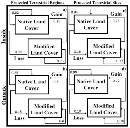
Figure 4 Probabilities of transition among types of land-cover change inside or outside of PAs, PTRs and PTSs.
Extreme PTSs were associated to areas with modified native cover from 1986 to 2011, where richness of subaquatic (Fig. 4i), tolerent (Fig. 4h) and tolerant (Fig. 4h) was higher, as well as groups of intermediate richness of pteridophytes (Fig. 4j) and gastropods (Fig. 4k). High and medium PTSs were associated to native land-cover from 1986 to 2011, containing groups of aquatic strictly with intermediate richness, lower subaquatic-tolerant richness, highest richness of pteridophytes and gastropods. The probability of recurrence of native land-cover was higher inside of PTRs than outside, the loss probability of native land-cover was higher outside of PTRs, while gain and modified land-cover were similar inside and outside of PTSs (Fig. 4c, d).
The type of change of PAs-PTRs and PTSs were different in function of fire, socioeconomic and topographic in 1986-2002 (Wilks lambda = 0.61, Wilks lambda = 0.5, respectively, Table 5) and 2002-2011 (Wilks lambda = 0.69, Wilks lambda = 0.53, respectively, Table 5). Comparison of land-cover change between 1986 and 2002 in PAs-PTRs showed that inside and outside modified land-cover presented similar characteristics, but these areas differ from other types of change (Fig. 5a). The risk of loss of native cover increases when the distance to agricultural areas decreases, native areas occur at an average distance of 4.3 km, while modified areas were at 0.3 km. Areas of loss-native between 2002 to 2011 in PAs- PTRs present similar distances to localities, agricultures, slope and elevations, and these types of change differ from areas with native land-cover. Modified, loss and gain land- cover occur at 0.3 km from agricultural areas, while native land-cover occurs at 3.5 km (Fig. 5b, Table 5).
Table 4 Compositions of rate land-cover changes inside and outside PTSs.
| Position | TPS | 1986-2002 | 2002-2011 | Wilcoxon test |
| Outside | Extreme | -0.638 | -1.14 | 0.0 |
| (p = 0.1) | ||||
| High | -2.702 | -4.85 | ||
| Medium | -2.535 | -4.55 | ||
| Total | -2.208 | -3.96 | ||
| Inside | Extreme | -0.840 | -0.48 | 0.0 |
| (p = 0.1) | ||||
| High | -4.015 | -0.82 | ||
| Medium | -4.225 | -0.70 | ||
| Total | -3.787 | -0.70 | ||
| Total | 0.0 | 3.0 | ||
| (p = 0.1) | (p = 0.28) |
Table 5 Factor structure of comparison of socioeconomic and environmental characteristics among type of land-cover change inside and outside of PTR and PTS. Significant probabilities in bold.
| Variables | Protected Terrestrial Regions | Protected Terrestrial Sites | ||||||
| 1986 - 2002 | 2002-2011 | 1986 - 2002 | 2002-2011 | |||||
| Root 1 | Root 2 | Root 1 | Root 2 | Root 1 | Root 2 | Root 1 | Root 2 | |
| DA1986 | 0.81 | 0.41 | NA | NA | -0.78 | 0.45 | NA | NA |
| DA2002 | 0.84 | -0.34 | 0.91 | 0.32 | -0.88 | -0.27 | -0.90 | 0.02 |
| DA2011 | NA | NA | 0.89 | 0.30 | NA | NA | -0.88 | -0.28 |
| DL1995 | 0.59 | 0.01 | NA | NA | NA | NA | NA | NA |
| DL2000 | NA | NA | 0.58 | -0.02 | -0.64 | 0.08 | -0.63 | 0.09 |
| DL2010 | NA | NA | 0.55 | -0.12 | NA | NA | NA | NA |
| Elevation | 0.47 | -0.21 | 0.51 | -0.56 | -0.52 | -0.05 | -0.54 | 0v.16 |
| D_fire | 0.52 | -0.08 | 0.56 | -0.36 | -0.31 | -0.18 | -0.36 | -0.07 |
| DHM1995 | 0.60 | 0.00 | NA | NA | -0.42 | 0.07 | NA | NA |
| DHM2000 | NA | NA | NA | NA | NA | NA | -0.63 | 0.08 |
| DHM2010 | NA | NA | NA | NA | NA | NA | -0.29 | -0.26 |
| Slope | 0.38 | -0.15 | 0.40 | -0.17 | -0.49 | -0.10 | -0.51 | -0.01 |
| Eigenvalue | 0.40 | 0.11 | 0.37 | 0.02 | 0.59 | 0.12 | 0.55 | 0.14 |
| % variance explained | 72.5 | 92.2 | 89.5 | 92.5 | 76.5 | 92.3 | 72.8 | 92.0 |
| F | 9.6 | 8.4 | 13.5 | 11.7 | ||||
| Degree of freedom | 494,736 | 424,379 | 494,989 | 565,288 | ||||
| p | < 0.0001 | < 0.0001 | < 0.0001 | < 0.0001 | ||||

Figure 5 Canonical position of centroids of type of land-cover change change (native = N, modified = M, loss = L, and gain = G) obtained from discriminant function analyses in 1986-2002 (a, d) and 2002-2011 (b, c) periods inside (I) and outsie (O) of PAs, PTRs and PTSs.
Comparisons of types of land-cover between 1986 to 2002 in PTSs show that native land-cover differs from areas with modified, loss and gain land-cover. Native cover occurs at 3.5 km from agricultural areas, to 3 km from the localities of 2000, and a slope of 10%; while areas with loss of native cover were to 1.9 km from agricultural areas; modified and gain of native cover areas were to 0.2 km from agricultural (Fig. 5c, Table 5). Finally, between 2002 and 2011, topographical and socioeconomic characteristics were similar inside and outside of PTSs, except to native land-cover. Native land- cover was outermost from agriculture areas (2.9 km), at slope of 7% and an elevation average of 600 m (Fig. 5c, Table 5).
Discussion
Relating diversity to land-cover changes inside and outside of PAs-PTRs-PTSs enables the prioritization of areas for conservation. Our study includes 5 groups of species that responded differently to the same environmental characteristics. Higher richness of aquatic plants occurs on the periphery of PTRs than the richness that occurs below 900 m asl, while higher ferns and gastropods richness occured inside of PTRs. However, outside of PTRs is where the rate of loss was higher. In contrasts, inside of extreme and high PTSs presented both richness of aquatic herbaceous species as rate loss of native land-cover. The loss of native land-cover increased by decreasing the distance to agricultural areas. Therefore, it is necessary to implement conservation strategies in areas with native cover near agricultural areas, since they are at greater risk of loss of native cover and contain a higher richness.
The highest hydrophyte and pteridophyte richness were associated with native land-cover loss, which is not the case for gastropod species. Therefore, the loss of coverage may affect the species that coexist in an area differently because each species requires specific environmental features (Venegas-Barrera et al., 2015). For example, pteridophytes are more common in temperate areas with flat slopes and environments with greater forest cover that favor shading (Bergeron & Pellerin, 2014). By contrast, aquatic plants require open, plains, and warm areas with little forest cover that can be flooded by water (Mora-Olivo & Villaseñor, 2007). These requirements also reflect the heliophilous characteristics of a vast majority of hydrophytes that inhabit large areas of open water lakes and other water bodies (Sculthorpe, 1985). We propose that conservation strategies must be expanded outside of PTRs, principally in PTRs surrounded by flat and tropical areas, where human activities are supported.
The loss of native cover is one of the greatest risk factors to PAs worldwide and occurs more frequently in the tropics (Lambin et al., 2001, 2005; Le Saout et al., 2013; Leisher et al., 2013). Natural cover losses within PAs occur in different countries around the world; estimates of annual losses of native coverage range from 1 to 9% of the total area of a PA. Higher rates of change in PAs occur in Malaysia, Indonesia, Botswana, Mexico and Guatemala (Bertzky et al., 2012; IUCN, 2005; Leverington et al., 2010; Nagendra, 2008). Although there is a loss of land-cover inside PAs, the land-cover losses are more evident on the periphery, due to limited legislation that regulate these areas (Halffter, 2011). In the present study, we found that the magnitude of the loss of coverage was different among the PTRs and PTSs, where the loss was more severe in the PTRs that were surrounded by flat zones (such as the Sierra de Tamaulipas or El Cielo) than in the PTRs with high slopes, such as Puerto Purificación and San Antonio Peña Nevada, and extreme PTSs.
We found that a higher richness and loss of land-cover frequently occurs in flat areas located on the peripheries of PTRs, whereas lower richness values of the 5 groups of species occur at elevations above 900 m asl, where PTRs show lower rates of loss of natural cover. The tropical lowland forest and scrubland vegetation types presented the highest loss of vegetation cover. Land-cover loss was strongly associated with areas of higher richness of pteridophyte and hydrophyte species. Our results showed that PTRs on steeper slopes showed lower loss of coverage, both inside and on the periphery, as well as in Puerto Purificación. PTRs surrounded by flat areas are more susceptible to the loss of native cover, such as Sierra de Tamaulipas. The loss of native cover in PAs is generated by human activities (as sugarcane crop, cattle farming) that occur on the peripheries, inducing changes in coverage of the PAs (Beresford et al., 2011; Bertzky et al., 2012; DeFries et al., 2007; Mas, 2005b; Smith, 2003). Examples of these changes are found in Egmont, New Zealand; Wolong, China; Yellowstone, USA; and Calakmul, Mexico, where land-cover losses occur more frequently on the peripheries, due to human activities (Bertzky et al., 2012; DeFries et al., 2007; Joppa & Pfaff, 2011).
Human activities were favored in flat areas or low slopes because these areas favor development of economic and social activities, as well as facilitate water supply (DeFries et al., 2007; IUCN, 2005; Joppa & Pfaff, 2011; Lambin et al., 2001; Leverington et al., 2010). However, some PAs include flat areas that are more likely to be affected by human activities (Halffter, 2011; McDonald et al., 2007). In Mexico, Los Tuxtlas and Montes Azules are PAs that have had the greatest losses of native land- cover. Moreover, these areas are mountainous regions surrounded by plains where human activities occur that facilitate land-cover loss inside the PAs. Los Tuxtlas, a mountain system surrounded by a leeward marine plain, is mainly affected by livestock production (Figueroa & Sánchez-Cordero, 2008; Halffter, 2011; Urquiza-Haas, 2009; Von Thaden et al., 2018). In our study, distinctive areas of strict, subaquatic and tolerant aquatic species show a similar pattern, where higher richness occurred outside of PTRs and PAs with flat lands, and medium richness was frequent at medium elevations and lower richness at higher elevations. In contrast, ferns and gastropods showed that higher richness occurs at elevations above 1,200 m asl and lower richness at elevations below 900 m asl.
In Mexico, the connectivity among protected areas is lower (Santini et al., 2016), where less than 4% of PAs are connected (Saura et al., 2018). Therefore, it is necessary to implement conservation strategies that reduce the loss of land-cover in flat areas to favor the persistence of land-cover and advocate connections with other PAs, principally in native cover near to agricultural areas (Hansen & DeFries, 2007; IUCN, 2005; Joppa & Pfaff, 2011; Leverington et al., 2010; Mas, 2005b; McDonald et al., 2007; Nagendra, 2008). The future scenarios proposed by Semarnat (2012) indicate that the areas with the highest risk of coverage losses are in Sierra de San Carlos and Sierra de Tamaulipas. The reduction in land-cover in Tamaulipas can be due to various socioeconomic processes, such as an increase in ecosystem restoration and a shift in environmental policies to promote land-use and land-cover change (Velázquez et al., 2002).
Our results suggest that the biggest loss of land-cover occurs on the periphery of the Sierra de Tamaulipas and El Cielo. If the degradation process continues in Sierra de Tamaulipas, then further isolation may occur compromising the persistence of species that require a combination of environmental attributes to complete their life cycles. Sierra de Tamaulipas is characterized by a mountainous area located in the coastal plains of Tamaulipas and is surrounded by the biogeographic province of the Gulf of Mexico (Cotler, 2010). Development of urban and agricultural activities is favored on the coastal plain, so the land-cover surrounding this area is among the most affected (IUCN, 2005). The dominant vegetation types in Sierra de Tamaulipas are tropical lowland forests and scrublands, which are the vegetation types that have experienced the greatest losses around the world and are the most sensitive to alterations (Pau et al., 2011).
Biodiversity loss is one of the consequences of land-cover loss that results in the isolation of populations and prevents the movement of species between different areas, which decreases gene flow and population viability (Mas, 2005a; McDonald et al., 2007; Nagendra, 2008). Major changes in land-cover have occurred in areas with high diversity and where the availability of resources has encouraged anthropogenic activities (de Lima et al., 2013). Therefore, identifying the impacts of land-cover losses in areas with higher species richness can be used to prioritize conservation areas. However, an important area of biodiversity is on the periphery of these areas (Bajracharya & Dahal, 2008; Bertzky et al., 2012; Ferreira et al., 2013). Less than 50% of vegetation types are accounted for in the Mexican PAs system, the remaining types occur on the peripheries of these areas (Urquiza-Haas, 2009). An evaluation of the richness of the other groups in these areas will permits the identification of areas where conservation strategies are a priority.
Social characteristics were related to land-cover changes in both periods, where change in native cover increased in areas near to agriculture areas (less to 0.2 km). Several studies have proposed that poverty increases deforestation, due populations with high or very high social marginality that invade, slash, and burn the forest nearest these localities (Lambin et al., 2001). We found that social marginality was less related to change; however, PAs nearest to localities had increased land-cover change risks. Therefore, it is necessary to promote conservation strategies to maintain these areas with high richness, through reforestation, maintenance of native landscapes, and increases in these areas to fill conservation gaps (Conanp, 2015; Mascia & Pailler, 2011). In this study, the application of a multidisciplinary statistical method combined with geographic information systems served as a tool to identify areas with greater richness that were affected by changes in coverage. Moreover, these areas were found to be suitable for preservation. The results of this analysis will be used to create strategies that contribute to the well-being of society and economic progress (Joppa & Pfaff, 2011; Leverington et al., 2008, 2010; Nagendra, 2008).
The cartography used in this study was acquired from INEGI and was generated by many methods at a scale of 1: 250,000. These conditions can result in the misclassification of many types of vegetation. Therefore, we recommend the use of land maps at a higher spatial resolution and standardized land-cover classification methods to obtain comparable and accurate data. The use of multi-criteria/multi-objective studies with the purpose of identifying and prioritizing the productive potential of soil is recommended to determine the sustainable use of natural resources (Noss et al., 2002). The methods used in this study represent a simple way to analyze priority regions and estimate the effects of land-cover changes on important species that require conservation.
Sierra of Tamaulipas was declared a PAs in 2016. However, the perimeter of the PAs is 8.5% smaller than the polygon of the PRs and only covers the areas that have remained unchanged in the coverage. Therefore, is necessary to extend the PAs to recover damaged areas and include the populations that are within its periphery. Finally, PAs and PTRs were areas where loss of native cover was lower but presented a lower richness; while PTSs present a higher loss native cover but high richness. We propose that new PAs should be considered to include other species different to endangered or at risk, as key, umbrella or dominant species, which will allow us to improve our strategies for the conservation of natural resources.

