


 nova página do texto(beta)
 Inglês (pdf)
 Artigo em XML
 Referências do artigo
 Enviar este artigo por email
 Citado por SciELO
  Similares em
SciELO
Similares em
SciELO 
 Permalink
Introduction
Environmental deterioration demands better documentation of the planet's biodiversity. This has required the development of tools that facilitate data management and decision-making, such as geographic information systems (Ferrier, 2002; Guisan & Theurillat, 2000; Guisan & Thuiller, 2005), which allow inferences about the distribution of a species or a group of species to be made more quickly and easily (Elith et al., 2006; Peterson & Soberón, 2012). Among the multiple uses of geographic information systems (GIS), there are studies in which they use these tools to model plant communities (Franklin, 1995). Predicting the distribution of a plant community using GIS has been important in studies of conservation of priority areas, of ecological restoration and to evaluate the effect of climate change (Bojórquez-Tapia et al., 1995; Franklin, 1995; Zimmermann, 2000).
The geographical limits of a plant community are not always easy to define (Méndez-Toribio et al., 2014). In studies that model communities, several strategies have been proposed for identifying the spatial patterns that define them (Elith et al., 2006; Ferrier, 2002; Ferrier & Guisan, 2006; Franklin, 1995). One of the most used methodologies in the modeling of the distribution of plant communities is using species assembly, which consists of the combination of individual potential distribution models to generate a map of the distribution of a community. This combination provides information on the distribution of species richness in certain areas within the study community. In addition, it allows the identification of spatial patterns followed by the species that make up this community (Ferrier & Guisan, 2006; Franklin, 1995; Guisan & Zimmermann, 2000).
The different methodologies and algorithms used to model the potential distribution of species yield different results (Araújo & Guisan, 2006; Elith et al., 2006; Pearson et al., 2006). For this reason, alternative statistical tests have been implemented to evaluate the performance of the models, such as the binomial test, the partial ROC (receiver operating characteristics), the AUC (area under the curve), etc. (Fielding & Bell, 1997; Hirzel et al., 2006; Liu et al., 2016; Oreskes et al., 1994; Peterson et al., 2008). These statistics use a set of data independent from the data used to generate the model to evaluate the performance and constancy of a model. Model evaluation allows researchers to discern which model is the most appropriate and best supported by the observed data (Johnson & Omland, 2004), guaranteeing the correct interpretation and quality of the results (Guisan & Thuiller, 2005; Mateo et al., 2011; Muñoz & Felicisimo, 2004). Despite the importance of these tests, such validation with independent data (some set of data not used as training or test) is rarely used in species modeling studies.
The seasonally dry tropical forest (SDTF), also known as tropical dry forest, is considered one of the most diverse and distinctive biomes worldwide due to the large number of endemic species it harbors (Olson et al., 2000). In Mexico, SDTF contains more than 6,000 species of vascular plants, of which more than 40% are endemic (Rzedowski, 1978; Villaseñor & Ortiz, 2014). National states with the highest number of endemic or characteristic (mostly restricted to) SDTF species are Oaxaca (1,396), Guerrero (1,251), Jalisco (1,237), and Michoacán (1,053; Villaseñor, 2016). In Michoacán, SDTF is located mainly in the Balsas Depression, a physiographic and floristic province that also contains the largest area of SDTF in the country (Rzedowski, 1978). The SDTF in the state of Michoacán contains 18% of the total vascular flora reported for the state (Villaseñor, 2016).
For several decades, the SDTF has faced serious conservation problems due to urban expansion and the constant exploitation of plant and animal species. As such, its original distribution area has been drastically reduced, causing the loss of and constant threat to a high number of species, mainly endemic. Due to this problem, it is considered among the most threatened tropical biomes in the world (DRYFLOR et al., 2016; Challenger & Soberón, 2008; Trejo & Dirzo, 2000).
This study has the purpose of evaluating different proposals of the potential distribution of the SDTF in Mexico, specifically in the state of Michoacán. In Mexico, STDF includes low deciduous forest, deciduous tropical forest, dry forest, and thorny forest (Miranda & Hernández, 1963; Rzedowski, 1978; Villaseñor & Ortiz, 2014) and is distributed mainly in the Pacific slope from southern Sonora and southwestern Chihuahua to Chiapas and on the gulf slope from Tamaulipas to the Yucatán Peninsula. It is found at altitudes ranging from 0 m to 1,900 m (Villaseñor & Ortiz, 2014). An important determining characteristic of STDF distribution is temperature, particularly the extreme minimum temperature (Challenger & Soberón, 2008).
Michoacán, with 1,053 species of native plants mostly distributed in the SDTF, ranks fourth in richness at the state level. In addition, several floristic studies have documented a large part of the flora and its biodiversity in general (e.g., Cué-Bär, Villaseñor, Arredondo et al., 2006; Cornejo-Tenorio & Ibarra-Manríquez, 2017; Leavenworth, 1946; Rodríguez & Espinosa, 1995, 1996), information that allows inferences to be made about the distribution of species among different biomes. Given the number of species present in the SDTF and the information available (databases with enough information to develop ecological niche models), it is important to evaluate the hypothesis that flowering plants (Angiosperms) that are endemic to Mexico, whose distribution is restricted to the SDTF, are good predictors of its geographical distribution.
The delimitation of the SDTF in Mexico has been addressed several times using GIS that consider different inputs, including the combination of plant and animal species (Prieto-Torres & Rojas-Soto, 2016), empirical knowledge (Rzedowski, 1990), vegetation censuses (INEGI, 2003) or particular plant species (Villaseñor & Ortiz, 2014). However, to date there has been no evaluation of these proposals to define which model is more statistically accurate in delimiting the biome.
The objective of this work is to propose a delimitation of the SDTF in the state of Michoacán based on the assembly of ecological niche models of species that proposals that delimit the biome, such as Rzedowski (1990), INEGI (2003), Villaseñor and Ortiz (2014) and Prieto-Torres and Soto-Rojas (2016).
Materials and methods
The endemic or characteristic (mostly restricted to) species of the seasonally dry tropical forest (Villaseñor, 2016, unpublished data) in Michoacán were selected based on the number of records from 2 sources of information: the National Biotic Information System (SNIB-REMIB) at the Comisión Nacional para el Conocimiento y Uso de la Biodiversidad (Conabio, 2018), and the digital repository of the National Herbarium of Mexico (MEXU-UNIBIO), at the Instituto de Biología, Universidad Nacional Autónoma de México (UNAM). The selected records were stored in a database which was later refined following the recommendations of Castillo et al. (2014) and Chapman (2005). Namely, 1) duplicate records were eliminated, 2) records that did not have coordinates were georeferenced, 3) records that could not be georeferenced were deleted, and 4) species with < 5 records were excluded (Pearson et al., 2007). The final database consisted of 76 species. Finally, for each species, an exploration of the data was carried out by generating their biogeographic track in ArcMap using the tool “minimum spanning tree tools”/ EMST in order to detect sampling points of a species that deviate from the geographical pattern followed by most of the records. Any disjoint points detected were carefully evaluated, both taxonomically and geographically, for inclusion or elimination in the analyses (Fig. 1).
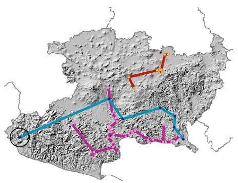
Figure 1 Biogeographic tracks of 3 species endemic or characteristic of the seasonally dry tropical forest. Notice that species with a blue line shows a site (black circle) which departs significantly from the pattern followed by the track in the study area (Michoacán).
We considered 58 environmental variables, with a resolution of 30 seconds (~1 km2), obtained from different sources. Twenty-six variables are climatic (Hijmans et al., 2005; Cruz-Cárdenas, López-Mata, Villaseñor et al., 2014), 9 topographic, 9 edaphological and 14 include remote sensing data (Cruz-Cárdenas, López-Mata, Ortiz- Solorio et al., 2014). The 58 layers were cut using the polygon of the state of Michoacán as a mask; the clipping of the variables was carried out in ArcMap 10.0 (ESRI, 2010). Restriction of the variables to the limits of the state of Michoacán was done in order to represent more precisely the accessible area (M in the BAM diagram) that a certain species can occupy (Soberón & Peterson, 2005; Soberón et al., 2017), thus improving model calibration (Barve et al., 2011).
The use of too many environmental predictors can cause overfitting of the models, leading to errors in the prediction of species distributions (Peterson & Nakazawa, 2008). To reduce the number of variables, a Principal Component Analysis (PCA) was carried out (Dormann et al., 2007). For this analysis, the values of the 58 variables were extracted from each of the presence records; these values were used to run a PCA in R program (R Development Core Team, 2017). The components that accumulated 80% of the variance, and within each component, the variables with above 95% of the load values were used for further analyses. The PCA made it possible to detect the components with the greatest contribution to the models and eliminate collinearity among the variables (Cruz- Cárdenas, López-Mata, Villaseñor et al., 2014).
An ecological niche model was constructed individually for each of the selected endemic/characteristic SDTF species. Niche models were generated using Maxent's algorithm ver. 3.3.3e (Phillips et al., 2006), which uses only presence data to model the most uniform distribution of a given species throughout the study area, restricted by the environmental specifications of the presence data. The extrapolation of these values to a given area results in a probability distribution map ranging from 0 to 1 (Phillips & Dudík, 2008). Maxent has proven to be a reliable algorithm and generates good results even with small sample sizes (< 10) (Pearson et al., 2007; Phillips et al., 2006).
The inputs used to run the ecological niche models were the records of the presence of each species and the environmental variables with the greatest contribution in the PCA. The program was used with the default configuration except for the do clamping and extrapolate option, to avoid extrapolation of the extreme values of the variables (Elith et al., 2011). It was also configured to use 25% of the data to validate the model and 75% to run the analysis (Phillips et al., 2006). Individual models were evaluated using independent threshold statistics, such as the Area under the curve (AUC), although it has been strongly criticized for the similar weight attributed to omission and commission errors (Lobo et al., 2008; Peterson et al., 2008). Therefore, in addition the models were also evaluated using the partial ROC (Peterson et al., 2008) which was calculated with the tool for partial ROC V. 1.0 program (Barve, 2008), applying 1,000 iterations and considering 5% error. The significance of the AUC ratio was estimated with bootstrapping (1,000 replications) using 50% of training localities; such AUC ratios were calculated with the Z test of the R program (http://www.r-project.org/).
The Maxent logistic outputs from each of the 76 species-level ecological niche model were processed in ArcMap ver.10.0, to obtain the potential distribution of the SDTF. The probabilistic models obtained from Maxent were converted to binary layers (0-1) using the maximum training sensitivity plus specificity threshold, which has been shown to be the most accurate in predicting the distribution of species (Jiménez-Valverde & Lobo, 2007; Liu et al., 2013; Weber, 2011). The resulting binary models were summed using the Algebra map tool implemented in ArcMap (D'Amen et al., 2015, 2017; Henderson et al., 2014). The layer with the sum of the models was reclassified using 76 thresholds, each representing the superposition from 1 to 76 of the individual models. At each threshold errors of omission were calculated considering all the records of the modeled species plus an additional number of data documenting the presence of the STDF in Michoacán. An error of omission was considered when a point of presence of the species was not predicted by the threshold (Fielding & Bell, 1997). The threshold with the lowest error rate of omission was considered as the potential distribution of the STDF in Michoacán.
The comparison and evaluation of the different models of the distribution of the SDTF was carried out using several statistical tests. These tests also allowed to evaluate the over- and under-estimation of the proposals of the STDF distribution. The following proposals were compared to the model generated in this study: Rzedowski (1990), INEGI (2003), Villaseñor and Ortiz (2014), and Prieto-Torres and Soto-Rojas (2016). The first test was a comparison of the geographic overlap between our model and each of the previous models, calculated by adding each pair of models using the “Algebra map tool package” of ArcMap. In a second test, the similarity of the models was evaluated using the Kappa estimator. For this analysis, our model was considered the closest to the potential distribution of the SDTF (reference model). The analysis was performed with the Kappa Analysis Tools extension in ArcView 3.x (Jenness & Wynne, 2005, 2007; Pontius & Millones, 2011). This estimator measures the overall similarity of the model, considering a rank from 0-1, in which values < 0.40 are considered bad models, < 0.60 regular models, > 0.80 good and 1 excellent (Landis & Koch, 1977).
A third evaluation test consisted of quantifying errors of omission, using all the presence records of the selected species. The presence data points were superimposed on each of the 4 models to identify where the models failed to predict them. A fourth evaluation analysis was a binomial test using 183 additional records of species of vascular plants characteristic of the SDTF that were independent of the points used to generate the model. This test gives an estimate of the amount of omission errors of each proposal. Finally, 2,320 occurrence records of species (Conabio, 2018) reported in vegetation types adjacent to the SDTF were used to obtain the model with the greatest uncertainty in the classification of the biome. These vegetation types were tropical sub-deciduous forest (373 records), Quercus forest (1,806), humid mountain forest (118) and xerophytic scrub (23). This final test allowed the detection of over- and under- estimation by the models and the rate of commission errors.
Results
We documented 253 species recorded as endemic to or characteristic of (mostly restricted to) the SDTF in Mexico and occurring in Michoacán; in total they included 2,781 records. Of these species, 76 species had more than 5 records in the state, totaling 1,051 records that were used for modeling of the distribution of STDF in Michoacán (Table 1).
Table 1 Species used for the delimitation of the seasonally dry tropical forest in the state of Michoacán, Mexico (N = 76). For each species, the number of records used for training and test is indicated; likewise, the performance value of the model estimated through the AUC and Partial ROC, and the omission of the binary model (expressed as the number of records omitted) are indicated.
| Species | Training/testing | AUC | Partial ROC | Omission |
| Acanthaceae | ||||
| Aphelandra lineariloba Leonard | 6/1 | 0.938 | 1.333 | 1 |
| Dicliptera haenkeana Nees | 7/2 | 0.942 | 1.285 | 1 |
| Tetramerium langlassei Happ | 5/1 | 0.835 | 1.193 | 0 |
| Tetramerium rubrum Happ | 6/1 | 0.913 | 1.152 | 1 |
| Apocynaceae | ||||
| Fernaldia asperoglottis Woodson | 11/3 | 0.912 | 1.132 | 1 |
| Marsdenia callosa Juárez-Jaimes & W.D. Stevens | 5/1 | 0.977 | 1.509 | 0 |
| Prestonia contorta (M. Martens & Galeotti) Hemsl. | 5/1 | 0.901 | 1.127 | 0 |
| Thevetia pinifolia (Standl. & Steyerm.) J.K. Williams | 5/1 | 0.982 | 1.148 | 1 |
| Aristolochiaceae | ||||
| Aristolochia mutabilis Pfeifer | 4/1 | 0.956 | 1.733 | 0 |
| Asteraceae | ||||
| Bidens mexicana Sherff | 4/1 | 0.963 | 1.385 | 1 |
| Cosmos pacificus Melchert var. pacificus | 6/1 | 0.950 | 1.297 | 1 |
| Cymophora accedens (S.F. Blake) B.L. Turner & A.M. Powell | 4/1 | 0.998 | 1.637 | 1 |
| Dendroviguiera puruana (Paray) E.E. Schill. & Panero | 8/2 | 0.959 | 1.052 | 1 |
| Guardiola pappifera Paul G. Wilson | 3/1 | 0.993 | 1.518 | 1 |
| Melampodium dicoelocarpum B.L. Rob. | 9/3 | 0.917 | 1.366 | 1 |
| Melampodium nutans Stuessy | 9/2 | 0.962 | 1.153 | 1 |
| Pectis decemcarinata McVaugh | 12/3 | 0.980 | 1.181 | 0 |
| Pectis linifolia L. var. hirtella S.F. Blake | 9/3 | 0.887 | 1.335 | 1 |
| Boraginaceae | ||||
| Cordia globulifera I.M. Johnst. | 9/2 | 0.905 | 1.271 | 0 |
| Burseraceae | ||||
| Bursera confusa (Rose) Engl. | 8/2 | 0.849 | 1.156 | 2 |
| Bursera coyucensis Bullock | 27/9 | 0.986 | 1.121 | 2 |
| Bursera crenata Paul G. Wilson | 38/12 | 0.970 | 1.052 | 4 |
| Bursera discolor Rzed. | 19/6 | 0.958 | 1.088 | 1 |
| Bursera excelsa (Kunth) Engl. var. acutidens (Sprague & L. Riley) McVaugh & Rzed. | 3/1 | 0.998 | 1.987 | 0 |
| Bursera fagaroides (Kunth) Engl. var. purpusii Brandegee) McVaugh & Rzed. | 9/2 | 0.901 | 1.183 | 0 |
| Bursera infernidialis Guevara & Rzed. | 21/7 | 0.988 | 1.079 | 3 |
| Bursera kerberi Engl. | 23/7 | 0.971 | 1.066 | 2 |
| Bursera occulta McVaugh & Rzed. | 3/1 | 0.996 | 1.907 | 0 |
| Bursera paradoxa Guevara & Rzed. | 18/6 | 0.982 | 1.138 | 2 |
| Bursera sarcopoda Paul G. Wilson | 10/3 | 0.905 | 1.401 | 1 |
| Bursera sarukhanii Guevara & Rzed. | 26/8 | 0.976 | 1.052 | 1 |
| Bursera toledoana Rzed. & Calderón | 6/2 | 0.984 | 1.332 | 0 |
| Bursera trifoliolata Bullock | 12/3 | 0.970 | 1.157 | 2 |
| Cactaceae | ||||
| Backebergia militaris (Audot) Bravo ex Sánchez-Mej. | 10/3 | 0.955 | 1.058 | 2 |
| Pachycereus tepamo Gama & S. Arias | 6/1 | 0.999 | 1.619 | 0 |
| Stenocereus chrysocarpus Sánchez-Mej. | 7/2 | 0.956 | 1.328 | 1 |
| Celastraceae | ||||
| Crossopetalum managuatillo (Loes.) Lundell | 13/4 | 0.932 | 1.060 | 3 |
| Convolvulaceae | ||||
| Calycobolus nutans (Moc. & Sessé ex Choisy) D.F. Austin | 6/1 | 0.900 | 1.525 | 0 |
| Cucurbitaceae | ||||
| Cucurbita argyrosperma K. Koch var. argyrosperma | 6/1 | 0.947 | 1.519 | 0 |
| Rytidostylis longisepala (Cogn.) C. Jeffrey | 8/2 | 0.878 | 1.087 | 2 |
| Cyperaceae | ||||
| Carex arsenei Kük. | 5/1 | 0.991 | 1.288 | 0 |
| Euphorbiaceae | ||||
| Euphorbia linguiformis McVaugh | 5/1 | 0.987 | 1.294 | 0 |
| Euphorbia umbellulata Engelm. ex Boiss. | 7/2 | 0.953 | 1.348 | 0 |
| Jatropha galvanii J. Jiménez Ram. & J.L. Contr. | 4/1 | 0.982 | 1.899 | 0 |
| Jatropha stephanii J. Jiménez Ram. & Mart. Gord. | 11/3 | 0.994 | 1.161 | 3 |
| Manihot tomatophylla Standl. | 14/4 | 0.928 | 1.121 | 2 |
| Fabaceae | ||||
| Acaciella igualensis Britton & Rose | 4/1 | 0.997 | 1.614 | 1 |
| Aeschynomene hintonii Sandwith | 4/1 | 0.990 | 1.351 | 1 |
| Aeschynomene paucifoliolata Micheli | 5/1 | 0.925 | 1.252 | 0 |
| Desmanthus interior (Britton & Rose) Bullock | 8/2 | 0.973 | 1.193 | 1 |
| Lonchocarpus balsensis M. Sousa & J.C. Soto | 13/4 | 0.946 | 1.104 | 0 |
| Lonchocarpus obovatus Benth. | 4/1 | 0.951 | 1.479 | 0 |
| Lonchocarpus schubertiae M. Sousa | 7/2 | 0.975 | 1.341 | 0 |
| Mimosa egregia Sandwith | 7/2 | 0.974 | 1.596 | 0 |
| Mimosa rhododactyla B.L. Rob. | 5/1 | 0.981 | 1.486 | 1 |
| Mimosa rosei B.L. Rob. | 16/5 | 0.969 | 1.127 | 1 |
| Mimosa tricephala Schltdl. & Cham. var. nelsonii (B.L. Rob.) Chehaibar & R. Grether | 5/1 | 0.878 | 1.204 | 1 |
| Lythraceae | ||||
| Cuphea lobophora Koehne var. elongate S.A. Graham | 7/2 | 0.946 | 1.343 | 0 |
| Malpighiciaceae | ||||
| Galphimia multicaulis A. Juss. | 9/3 | 0.928 | 1.482 | 0 |
| Galphimia paniculata Bartl. | 5/1 | 0.902 | 1.440 | 0 |
| Malvaceae | ||||
| Gossypium lobatum Gentry | 18/5 | 0.985 | 1.135 | 0 |
| Gossypium schwendimanii Fryxell & S.D. Koch | 6/2 | 0.999 | 1.336 | 2 |
| Gossypium trilobum (Sessé & Moc. ex DC.) Skovst. | 5/1 | 0.988 | 1.950 | 0 |
| Pavonia oxyphylla (DC.) Fryxell var. melanommata (B.L. Rob. & Seaton) Fryxell | 6/1 | 0.876 | 1.478 | 0 |
| Sida fastuosa Fryxell & S.D. Koch | 6/1 | 0.952 | 1.543 | 0 |
| Waltheria pringlei Rose & Standl. | 15/5 | 0.933 | 1.077 | 1 |
| Nyctaginaceae | ||||
| Salpianthus aequalis Standl. | 6/2 | 0.900 | 1.264 | 1 |
| Passifloraceae | ||||
| Passiflora juliana J.M. MacDougal | 3/1 | 0.990 | 1.869 | 1 |
| Passiflora viridiflora Cav. | 8/2 | 0.990 | 1.067 | 2 |
| Primulaceae | ||||
| Bonellia pringlei (Bartlett) B. Ståhl & Källersjö | 4/1 | 0.921 | 1.295 | 1 |
| Ranunculaceae | ||||
| Delphinium subscandens Ewan | 8/2 | 0.926 | 1.170 | 1 |
| Rhamnaceae | ||||
| Karwinskia johnstonii Ric. Fernández | 11/3 | 0.977 | 1.558 | 0 |
| Rubiaceae | ||||
| Simira mexicana (Bullock) Steyerm. | 9/2 | 0.971 | 1.215 | 1 |
| Santalaceae | ||||
| Phoradendron dolichocarpum Kuijt | 6/1 | 0.990 | 1.595 | 1 |
The principal components analysis applied to eliminate the collinearity of the variables indicated that the first 8 components explain 82% of the environmental variation, which included 30 of the 58 variables initially proposed (Table 2). Those 30 variables were used to run the ecological niche models for each species. A detailed explanation of the selected variables is provided by Cruz-Cárdenas, López-Mata, Villaseñor et al. (2014) and López- Mata et al. (2012).
Table 2 Variables used in the modeling of 76 species characteristics of the seasonally tropical dry forest in the state of Michoacán, Mexico.
| Type | Variable |
| Climatic | bio02 (average daytime variation) |
| bio04 (seasonality of temperature) | |
| bio05 (maximum temperature of the warmest month) | |
| bio06 (minimum temperature of the coldest month) | |
| bio07 (annual variation in temperature) | |
| bio11 (average of the coldest quarter temperature) | |
| bio12 (annual rainfall) | |
| bio13 (precipitation of the wettest month) | |
| bio15 (seasonality of precipitation) | |
| bio18 (precipitation of the warmest quarter) | |
| bio19 (precipitation of the coldest quarter) | |
| evahumed (real evapotranspiration of wet months) | |
| evasecos (real evapotranspiration of dry months) | |
| ppsecos (precipitation of dry months) | |
| Topographic | aspect (orientation 0° to 90°) |
| mexdem (digital model of elevation) | |
| mexslope (slope) | |
| tri (terrain roughness index) | |
| twi (topographic moisture index) | |
| Edaphic | mexca (calcium) |
| Cruz-Cárdenas, López-Mata, Ortiz-Solorio et al. (2014) | mexce (electric conductivity) |
| mexco (organic carbon) | |
| mexk (potassium) | |
| mexmg (magnesium) | |
| mexras (sodium absorption radius) | |
| *MODIS | modisdic (normalized vegetation index December) |
| modisfeb (normalized vegetation index February) | |
| modismar (normalized index of vegetation March) | |
| modisabr (normalized vegetation index April) |
* Variables obtained with remote perception data (MODIS web): Moderate Resolution Imaging Spectroradiometer; December, February, March, and April 2009.
An individual ecological niche model was generated for each of the 76 focal SDTF species. Most models had high AUC values (92%: 0.900-0.999, considered very good models). The remaining 8% of the models’ AUC values were considered good (0.835-0.0.887). The ecological niche models obtained were better than a randomly generated model (Baldwin, 2009; Peterson et al., 2011). Performance estimation of the models was also favorable using the partial ROC. Likewise, 100% of models were statistically significant, with AUC ratios ranging from 1.052 to 1.987 (p < 0.001; Table 1). The assembly of the binary models was considered to represent the potential distribution of the SDTF in Michoacán; the threshold limit of the SDTF was considered with the pixels where 5 or more species coincided, which was the cut-off threshold that produced the lowest percentage of errors of omission (17%).
The model of STDF distribution in the state of Michoacán generated here estimated a surface area of 22,483.3 km2, representing 38.7% of the state’s territory (Fig. 2). According to the model, SDTF is distributed mainly in the regions of the Balsas Depression and part of the Mexican Pacific Coast (Lázaro Cárdenas and Aguililla municipalities). Figure 2 shows the potential distribution of the SDTF in Michoacán and the number of species considered for its delimitation.

Figure 2 Potential distribution of the seasonally dry tropical forest (blue area) in the state of Michoacán obtained with the assembly of 76 individual species ecological niche models. The red circles show the occurrence points used in the modeling of the species considered.
The superposition (assembly) of the 76 models generated a detailed map of species richness along the distribution area of the SDTF (Fig. 3). The portions that concentrate more than 50% (29-43 species) of the species analyzed are found mostly in the southern and southeastern parts of the distribution, with an archipelago of small patches running to the northeast, near the state of Jalisco. The richest zones identified are included in 3 physiographic subprovinces (INEGI, 2014): the southern part of the Balsas Depression (the westernmost richest area), the Infiernillo Dam in Tierra Caliente (Southern Cordillera subprovince) near the border with the state of Guerrero, and the Tepalcatepec Depression at the western edge of the SDTF distribution, near the border with the state of Jalisco (Fig. 3). From these nuclei of high concentration of species, a gradient is formed that decreases towards the limits of the SDTF with other biomes, such as the temperate forest.

Figure 3 Number of species characteristic of the seasonally dry tropical forest (Table 1). The red color shows the areas of highest concentration of species (> 28), while the areas of lower concentration are shown in yellow.
Figure 3 shows the results of the comparison using the spatial coincidence, of the model proposed here (22,483.3 km2) with those proposed by Rzedowski (1990; 33,238 km2), INEGI (2003; 22,049 km2), Villaseñor and Ortiz (2014; 28,010 km2), and Prieto-Torres and Soto-Rojas (2016; 37,717 km2). The model with the largest coinciding area was that proposed by Prieto-Torres and Rojas-Soto (95%), and the model with the smallest coincidence was that of Villaseñor and Ortiz (78.4%). The models proposed by Prieto-Torres and Rojas-Soto (2016) and Rzedowski (1990) predicted larger areas, including many areas not included in our model (non-coincidence area), with 71.7% and 64.4% of overpredicted surface respectively (Fig. 4). Model evaluation metrics showed that the INEGI’s (2003) proposal is the most similar to ours, with a Kappa value of 0.54, considered a model fairly similar (Landis & Koch, 1977). At the other extreme, the model with the lowest similarity with respect to ours was that of Prieto-Torres and Soto-Rojas (2016), with a Kappa value of 0.34 (Table 3); in this case Kappa values refer to the similarity with respect to our model, not to the actual distribution of STDF.
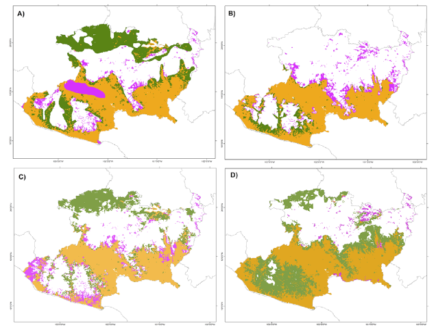
Figure 4 Comparison of the different proposals of distribution of the seasonally dry tropical forest in Michoacán with the potential distribution obtained in this study: A) Rzedowski (1990) model, B) INEGI (2003), C) Villaseñor and Ortiz (2014), D) Prieto-Torres and Soto-Rojas (2016). In all figures the orange color indicates the coincident areas, the lilac color indicates areas predicted by our model non-coincident with the proposed model, and the green areas the exclusive areas of each model not recorded by our model.
The model comparison based on omission errors using the 1,051 records of the 76 modeled species, indicated that proposal of Prieto-Torres and Soto-Rojas (2016) had the lowest omission rate (9.1%, 96 out of 1,051 records), followed by ours (16.8%, 177 records). The proposal with the highest rate of omission errors was that of Villaseñor and Ortiz (2014), with 19.7% (207 records, Table 3).
Table 3 Percentages of the statistical tests using 183 occurrence points of species characteristic of the seasonally dry tropical forest in Michoacán. These records were not used for models generation of the 76 species. The percentage of omission errors of each model is also indicated, considering in addition the total of points used to run the models.
| Models | Kappa | Binomial test | p-value < 0.5 | % Omission |
| Rzedowski | 0.35 | 0.62 | 8.80 × 10-07 | 18.36 |
| INEGI | 0.54 | 0.58 | 0.0001004 | 17.98 |
| Villaseñor and Ortiz | 0.41 | 0.55 | 0.001501 | 19.70 |
| Prieto-Torres and Soto-Rojas | 0.34 | 0.81 | 2.20 × 10⁻¹⁶ | 9.13 |
| This paper | 1.00 | 0.74 | 2.20 × 10⁻¹⁶ | 16.84 |
The binomial test carried out with 183 records that were not used to generate the models revealed that the 5 proposals resulted in probability values greater than 0.5 and were therefore better than a randomly generated model. The Prieto-Torres and Soto-Rojas (2016) model had the highest prediction probability (0.81, p-value < 2.20 × 10⁻¹⁶) and the model with the least predictive success was the one proposed by Villaseñor and Ortiz (2014) (0.55, p-value < 0.001). Our model had a prediction probability of 0.74 (p-value << 2.20 × 10⁻¹⁶). All models had high probabilities of classifying occurrences better than a randomly generated model (Table 3).
Table 4 shows how well the different models discriminated between SDTF and points of different vegetation types neighboring the biome. The models with the highest points’ misclassification were those proposed by Rzedowski (1990) and Prieto-Torres and Soto-Rojas (2016), 65.7% and 63.6%, respectively. Our model presented intermediate confusion (36%), compared to the other models. The model that presented the lowest commission error was INEGI (2003) with 14.8% confusion. The type of vegetation with the highest number of points erroneously classified as SDTF was Quercus forest.
Table 4 Collecting points classified as part of the biome by different proposals of distribution of the seasonally dry tropical forest. The number of erroneous points assigned to the biome per type of vegetation and the percentage of confusion considering the total points erroneously classified are indicated. BTSC = Tropical sub-deciduous forest; BQ = Quercus forest, BMM = humid mountain forest, MXE = xerophytic scrub.
| Models | BTSC (373) | BQ (1,806) | BMM (118) | MXE (23) | Total | % confusion |
| Rzedowski | 275 | 1,214 | 21 | 14 | 1,524 | 65.7 |
| INEGI | 368 | 19 | 1 | 7 | 345 | 14.9 |
| Villaseñor and Ortiz | 156 | 636 | 2 | 13 | 807 | 34.8 |
| Prieto-Torres and Soto-Rojas | 370 | 1,087 | 9 | 9 | 1,475 | 63.6 |
| This paper | 291 | 535 | 1 | 7 | 834 | 35.9 |
Discussion
The assembly of individual ecological niche models turned out to be a useful technique to find the environmentally suitable distribution of the SDTF in Michoacán. Such assembly of models is a widely used technique that identifies spatial patterns of species that characterize a community (Clark et al., 2014; D'Amen et al., 2015; Ferrier & Guisan, 2006; Franklin, 1995; Guisan & Zimmermann, 2000; Jiménez-Alfaro et al., 2018). A biome like SDTF is characterized by having well defined climatic conditions (Challenger & Soberón, 2008; Gurevitch et al., 2002); the species endemic or characteristic to it, due to their specific requirements, are good indicators of environmental conditions of the biome. One disadvantage attributed to this technique is that the community-level prediction can accumulate the errors from each individual model (Pottier et al., 2013). However, the assembly of models presents an important advantage in that the species that make up the community are identified, and therefore its composition is known, which for conservation issues is of great importance (D'Amen et al., 2015).
The use of species that are endemic to and characteristic of the SDTF in Michoacán to delimit its distribution resulted in a statistically well-supported model. This is mainly because the species considered are characterized by their specific environmental conditions; the smaller geographical ranges characterizing such species, offer complete scenarios about their distribution, allowing to capture more realistically the greater part of their environmental niche (Lomba et al., 2010). Lomba et al. (2010) discussed that the use species that are rare or have a restricted distribution, as is the case in species that are endemic or exclusive to a habitat, provides better projections across scales. These models with good predictive capacity lead to more accurate predictions about the dynamics of these species and the communities where they live.
In the geographical overlap test, although our model had a high degree of coincidence with that proposed by Prieto-Torres and Rojas-Soto (2016), the Prieto-Torres and Rojas-Soto model had a larger overestimated area. These authors included in their model species not restricted to the SDTF biome, such as Enterolobium cyclocarpum (Jacq.) Griseb. and Lysiloma divaricatum (Jacq.) J.F. Macbr., which are also recorded in contiguous temperate forests (Gopar-Merino & Velázquez, 2016). The use of widely distributed species can lead to multiple vegetation types being lumped together as one (Clark et al., 2014). The overestimation caused by the use of species with wide distribution increases the probability that when comparing an adjusted model characteristic of a biome, with a model in which species shows broad environmental conditions, results have greater coincidence in area. On the other hand, the overestimation observed in the proposals of Rzedowski (1990), INEGI (2003) and Villaseñor and Ortiz (2014), mostly observed in the southern and northwestern parts of the state, may be the result of errors due mainly to severely fragmented habitats (Mas et al., 2017), e.g. difficulty in distinguishing SDTF from secondary vegetation derived from SDTF or subtropical scrubs derived from Quercus forests (Challenger & Soberón, 2008; Trejo & Dirzo, 2000).
The Kappa statistics suggested that the model most like ours was the INEGI (2003) model. This statistic estimates classification errors when using one model to predict the other, so each of these models had a moderate capacity to predict the other, which involves both identifying the location of the SDTF as well as the omission and commission errors. On the other hand, the low value of Kappa for the model of Prieto-Torres and Soto-Rojas (2016), may be the result of high rates of commission errors with respect to our model, that is, a high percentage of area predicted by their model but not by ours. The high rates of commission errors translate into overestimation (Anderson et al., 2003), which in this case may be due to the use of widely distributed species to generate the model.
The omission error test favors the proposal of Prieto-Torres and Soto-Rojas (2016), inevitable with an overestimated model. The model had a larger total predicted area, increasing the probability of more points falling within the area proposed by this model, compared to tighter models such as the Rzedowski model (1990) and our model. The low rates of omission errors of Prieto-Torres and Soto-Rojas (2016) model with respect to ours, may also be due to the less restrictive threshold they used (“fixed omission value 5”) to obtain the binary models they used to determine the SDTF distribution. This lax omission value (0.05) contrasts with the more restricted values with which we convert the models to binary (minimum 0.09, maximum 0.7, average 0.4), which caused a higher rate of omission errors in our STDF model. Another test that also favors the proposal of Prieto-Torres and Soto-Rojas (2016) is the binomial test, also surely because the greater predicted surface increases the probability that more points fall within the area predicted by the model, and therefore more points are correctly classified when they should be considered incorrectly placed.
The commission errors test favors the INEGI (2003) proposal; this delimitation confuses the SDTF with other plant communities less frequently than the other models. In contrast, Rzedowski (1990) and Prieto-Torres and Soto-Rojas (2016) more frequently determine localities of other biomes as part of the SDTF (Table 4). It is likely that including more generalist and widely distributed species resulted in a higher percentage of commission errors (64%), when compared with localities of neighbor biomes (Table 4). For example, Cochlospermum vitifolium (Willd.) Spreng., Enterolobium cyclocarpum (Jacq.) Griseb., Haematoxylum brasiletto H. Karst., Ipomoea wolcottiana Rose, and Lysiloma watsonii Rose, used in model’s generation by these authors, are widely distributed in 3 or more biomes other than SDTF. These species’ models include environmental conditions from other biomes, mistakenly transferring these characteristics to the analysis and leading to an overestimated model.
Broadly distributed species are difficult to model because both their ecological and environmental characteristics affect the accuracy of the model compared to species of restricted distribution (Hernández et al., 2006; Segurado & Araujo, 2004; Thuiller et al., 2004). A high rate of commission errors can have negative consequences for conservation because they would be defining areas as potentially important for a species or a group of species when that species or group of species is not actually present (Kramer-Schadt et al., 2013). Accordingly, the appropriate selection of the species to be considered to model a plant community with specific characteristics can help to obtain more accurate conclusions (Aitken et al., 2007; Lomba et al., 2010; Mateo et al., 2011).
An additional problem with the comparison of proposals on the geographical definition of the SDTF is that the techniques applied are difficult to replicate. Sometimes the proposals have been elaborated based on the opinion and experience of a group of experts (for example Rzedowski, 1990), or require high investment and too much time to conduct vegetation censuses to define it, which are not always convincing due to non-uniformity in data collection (for example INEGI, 2003). Although the model of Prieto-Torres and Rojas-Soto (2016) was favored by the highest number of validation tests, it does not mean that it is the model that best represents the distribution of the SDTF in Michoacán. These tests favored this proposal because it was biased by the overestimation of the model by using species of wide distribution. The overestimation led to more successfully predicted points in the omission and binomial errors tests, but it also resulted in greater confusion and that records of species from other contiguous biomes were classified as SDTF. This made it the second- least adequate proposal (following Rzedowski’s) of the potential geographical distribution of SDTF in Michoacán.
Only 8.5% (2,856 km2) of the area with the highest concentration of species richness (> 28 species) is within a protected natural area (the Zicuirán-Infiernillo Natural Reserve). Given that SDTF is considered one of the most important and endangered biomes, especially due to its high degree of endemism (Cué-Bär, Villaseñor, Morrone et al., 2006; DRYFLOR et al., 2016; Olson et al., 2000), results discussed here can be used to make proposals for ANPs in the areas with the highest concentration of endemic species. There are currently no protected areas in the Balsas Depression and the Southern Coastal Range, where there was a high concentration of characteristic species.
Modeling the potential distribution of species at the community level allows for effective forecasting of factors that threaten biodiversity such as climate change, as well as providing knowledge on the functioning of the ecosystem (D'Amen et al., 2015). That is why it is important to make a rigorous selection of the species integrated to the algorithms for modeling the distribution of communities. The consideration of endemic and characteristic species of a plant community, described by its specific requirements (for example the SDTF), provide results closer to the observed data than those found when widely distributed species are considered. More precise models will surely allow for more accurate conservation proposals of potentially important areas due to their species richness.

