


 nueva página del texto (beta)
 Inglés (pdf)
 Artículo en XML
 Referencias del artículo
 Enviar artículo por email
 Citado por SciELO
  Similares en
SciELO
Similares en
SciELO 
 Permalink
Introduction
The diversity of coral reef communities has always been considered to be higher than other marine habitats (Emery, 1978). Although coral reef ecosystems cover less than 0.07% of the ocean surface, they are the home to 25% of all known marine species on the planet (Spalding & Brown, 2015; Spalding & Grenfell, 1997; Spalding et al., 2001). Calculations of the fish diversity in these ecosystems propose approximately 4,000 to 8,000 species, indicating that coral reef ecosystems are the host of one of the most diverse fish assemblages to be found anywhere on earth (Lieske & Myers, 2001; Spalding et al., 2001).
The Caribbean Sea is considered a unique biogeographic region and is among the top 5 world hotspots for marine biodiversity (Rivera-Monroy et al., 2004). It constitutes 12% of the total reefs of the world, shelters approximately 500 species of fishes, and presents the second largest reef barrier in the world, the Mesoamerican Barrier Reef System (MBRS) (Cortés, 2003; Hughes, 1994). Yet, over the last years, the Caribbean Sea is among the regions where the most serious declines in terms of reef area, health, and fisheries productivity is occurring (Gardner et al., 2003; Miloslavich & Klein, 2005).
Coral reefs around the world are under stress by the combined effect of negative factors. As a result of global climate change, we are facing issues such as ocean warming (Frieler et al., 2012; Roxy et al., 2016; Spalding & Brown, 2015) and acidification (Wisshak et al., 2012). Invasive species such as the lionfish (Pterois volitans) and seagrass species (Halophile stupulacea) are dramatically changing the trophic webs (Arias-González et al., 2011; Williams, 2007), and anthropogenic effects such as overfishing and pollution have severely degraded these ecosystems (Sandin et al., 2008).
Although coral reefs are in crisis worldwide (Bellwood et al., 2004; De’ath et al., 2012; Huang, 2012; Nyström et al., 2000), the response to stressors will vary depending on the resilience of these ecosystems (Roff & Mumby, 2012). In ecology, resilience is the capacity of an ecosystem to respond to a perturbation or disturbance by resisting damage and recovering (Folke et al., 2004). The analyses of functional groups, born as a way to measure the trophic web diversity of ecosystems (Petchey & Gaston, 2006), has shown that the level of redundancy within these functional groups can be a measure of reef assemblage stability, and ultimately a measure of coral reef resilience to perturbations (Clarke & Warwick, 1998; Nyström, 2006).
Functional groups are collections of species that perform a similar ecological function in the ecosystem, irrespective of their taxonomic affinities (Bellwood et al., 2004; Steneck, 2001; Steneck & Dethier, 1994). The ability of species to use specific resources in specific areas of the ecosystem relies on its morphological design (Fulton, 2007; Wainwright & Bellwood, 2002). Through the study of these strong relationships between habitat use, morphology, and diet on coral reef fishes, it is possible to recognize groups with highly specific niche and consequently, highly specific functions in the ecosystem (Aguilar-Medrano & Calderón-Aguilera, 2015; Aguilar-Medrano et al., 2011, 2012; Fulton, 2007; Wainwright & Bellwood, 2002).
Morphology has been used to aid in determining functional groups (Córdova-Tapia & Zambrano, 2016; Villéger et al., 2010), conditioning morphology to a number of measurements that we cannot readily visualize as descriptors of shape differences. Aguilar-Medrano and Calderón-Aguilera (2015) proposed a classification of functional groups based on diet and morphology, using geometric morphometrics to define shape variations. Geometric morphometric analyses not only solves many of the problems confronting traditional methods of measurement by offering precise and accurate descriptions, but also it serves the equally important purposes of visualization, interpretation, and communication of results (Zelditch et al., 2004). Thus, in order to study the relationship between fish functional groups and habitat complexity along the coast of the Yucatán Peninsula we have used the classification of Aguilar-Medrano and Calderón-Aguilera (2015).
For a long time researchers have investigated the relationship between fish species richness-diversity and habitat complexity variables such as topography, depth, substrate, slope, currents, and coral cover, among others (Aguilar-Medrano & Calderón-Aguilera, 2015; Arias-González et al., 2011; Carpenter et al., 1981; Dominici-Arosemena et al., 2005; Gosline, 1965; Harmelin-Vivien, 1977; Levin, 1993; Luckhurst & Luckhurst, 1978; McGehee, 1994; Roberts & Ormond, 1987; Williams, 1982). All variables have shown differences according to the region; however, habitat complexity and anthropogenic pressure appear to be the factors with the highest correlation to fish abundance and diversity (Arias-González et al., 2008, 2011; Bell & Galzin, 1984; De’ath et al., 2012; Huang, 2012; McCormick, 1994; Nemeth & Appeldoorn, 2009).
In the present study, we retrieve the dataset of Ruiz-Zárate and Arias-González (2004), collected during 1999 and 2000, including richness and distribution of fish and coral community, and the reef zones of the eastern coast of the Yucatán Peninsula, belonging to the north sector of MBRS (Fig. 1). By combination of these data and new information on diet and morphology of the fish community, we analyzed and classified into functional groups the coral reef fish community of the eastern coast of the Yucatán Peninsula. The aims of our study were: 1) determine the functional relationships of the fish community based on diet and morphology, and 2) determine the extent of the influence of habitat complexity and the protection of the Sian-Ka'an Biosphere Reserve on the richness of fish and the functional diversity of the ecosystem. The information obtained from our study will provide ecological tools for managers and politician to implement governance measures for the resilience of the MBRS.
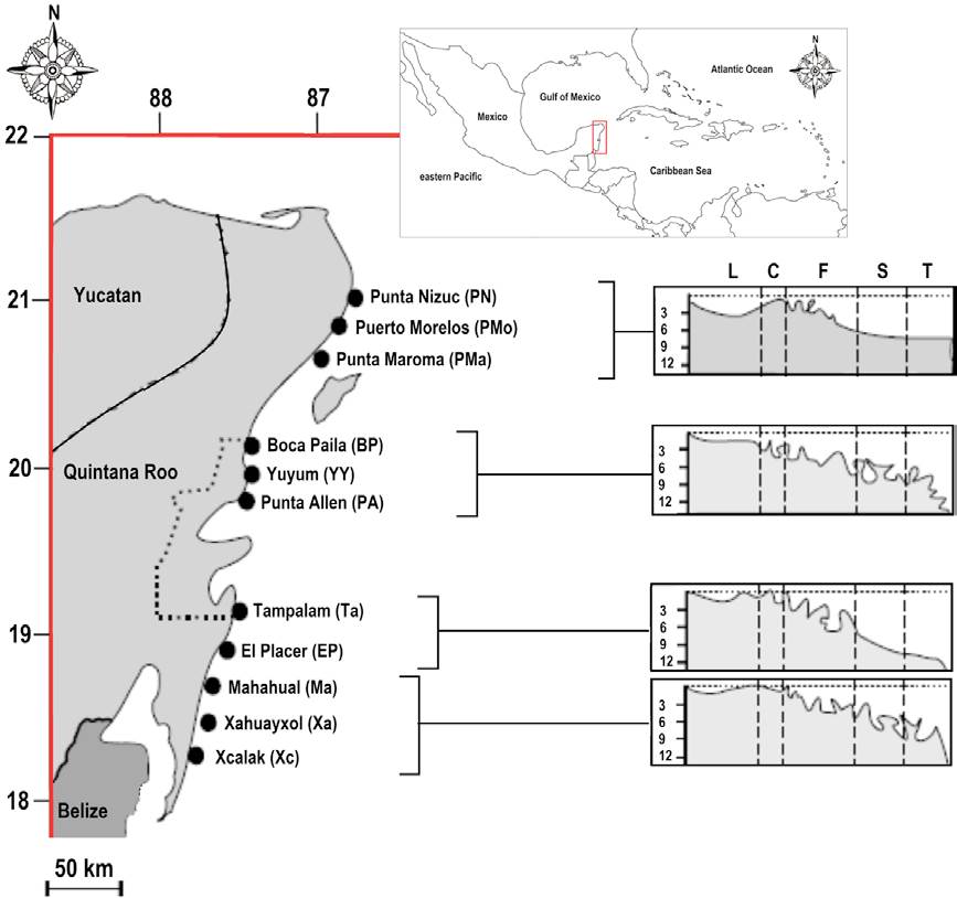
Figure 1 Study sites in the eastern coast of the Yucatán Peninsula, Mexico, belonging to the north sector of the Mesoamerican Barrier Reef. On the right, the 4 types of topographic profiles of the area. Reef division zones: L, reef lagoon; C, reef crest; F, reef front; S, reef slope; T, reef terrace. Numbers indicate depth in meters. The dotted area represents the Sian-Ka’an Biosphere Reserve.
Materials and methods
This study considered 11 coral reefs localities of the eastern coast of the Yucatán Peninsula. Reefs in this area show a gradient of anthropogenic pressure from north to south (Arias-González et al., 2008), with the Sian-Ka'an Biosphere Reserve in the central area (Fig. 1). Moreover, reefs show a clear geomorphologic zoning in 5 zones: lagoon, crest, front, slope (corresponding to the spore and grove), and terrace (Arias-González et al., 2008, 2011; Ruiz-Zárate & Arias-González, 2004); however, the crest zone is not considered in fish or coral censuses because is too shallow. For information on sampling design, see Arias-González et al. (2008) and Ruiz-Zárate and Arias-González (2004). Since fish species show trophic and morphological variation throughout their ontogeny, in this study we only considered adults specimens.
To determine the trophic level of each species in a numeric way, we used the troph index available in Fishbase (Froese & Pauly, 2016). Troph index is defined by 5 main categories: i) detritus: debris and carcasses; ii) plants: phytoplankton; iii) zoobenthos: sponges, cnidarians, worms, mollusks, benthic crustaceans, insects, and echinoderms; iv) zooplankton: jellyfish and planktonic crustaceans; and v) nekton: fish (early stages) and cephalopods (Froese et al., 1992). Accordingly, organisms consuming items from the first or/and second groups (detritus and phytoplankton) will present low troph values, while organisms that consume higher energy groups will present highest troph values. Troph index is calculated using qualitative information from the list of items known to occur in the diet of each species and results in a numerical value (Aguilar-Medrano et al., 2015; Costa & Cataudella, 2007).
Two linkage methods of cluster analysis were used to analyze trophic groups: 1) unweighted pair group method with arithmetic mean (UPGMA), using Euclidian distance. UPGMA is an agglomerative hierarchical clustering method that constructs a rooted tree that reflects the structure present in a pairwise similarity matrix (Sokal & Michener, 1958), and 2) Ward’s minimum-variance method, which is a clustering algorithm that optimizes based on within-group variance rather than raw distance (Ward, 1963). To choose the best linkage method we used Cophenetic correlation coefficient as measure of the goodness-of-fit of the dendrogram to the original data (Cardini & Elton, 2008; Sokal & Rohlf, 1962). All possible sets obtained from the cluster analyses were examined by multiple analysis of variance (Manova) and analysis of variance (Anova) to test whether the trophic groups were statistically different based on p values.
The mean standard length (SL) of each species was recorded from literature and the relationships between size and trophic values were tested by regression analyses.
On the eastern coast of the Yucatán Peninsula, from 1999 to 2000, 171 species were recorded. From these, 160 were used in this study. The rest were not included due to their morphological variation, which did not allow us to use the same landmark configuration used for the rest of the species. Among the species not included, there are cartilaginous fish (e.g., Ginglymostoma cirratum, Enchelycore nigricans, Dasyatis americana, Aetobatus narinari) and ray finned fishes (e.g., Stygnobrotula latebricola).
A total of 360 images, representing 160 species belonging to 40 fish families were analyzed. The images were collected from fish collections as SIO (San Diego, CA, USA), LACM (Los Angeles, USA), USNM (Washington, USA) and specialized web resources such as MorphBank (www.morphbank.net) and FishBase (Froese & Pauly, 2016).
Geometric morphometric methods were used to quantify shape and size variation (Bookstein, 1991; Rohlf, 1999; Rohlf & Marcus, 1993; Zelditch et al., 2004) in each trophic group. To capture as much shape variation as possible, 16 landmarks were recorded (Fig. 2). Configurations were optimally superimposed using a Generalized Procrustes analysis (Rohlf, 1999; Rohlf & Slice, 1990) to obtain a matrix of shape coordinates. Relative Warps including both uniform and non-uniform components (Bookstein, 1991; Rohlf, 1993) were calculated from the Procrustes data and used as shape variables for the statistical analyses. Finally, the centroid size (CS) was used as an estimate of size (Bookstein, 1991).
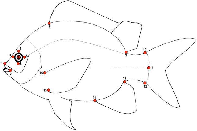
Figure 2 Landmarks used in geometric morphometric analyses: (1-2) snout, (3-7) eye, (8-9) dorsal fin, (10-12) caudal peduncle, (13-14) anal fin, (15-16) insertion of the pectoral fin.
To explore the main axes of shape variation among specimens a principal components analyses (PCA) was performed and to gain a better appreciation of the shape variation associated with the main axes of PCA, thin-plate spline algorithm (Bookstein, 1991) was used to produce transformation grids representing extreme positive and negative deviations along the axis.
First, trophic groups were tested for the presence of overall morphometric differences using one-way Manova and pairwise multiple comparisons using Hotelling’s T value with uncorrected significance. Next, the morphological variation within each group was explored by cluster analysis (UPGMA and Ward’s method) and PCA to determine the possible morphological sets. Finally, each morphological set was tested by analyses of variance as canonical variance analysis (CVA), Manova, and Anova.
The effect of habitat complexity (coral cover and number of reef zones), and the protection of the reserve (localities inside the Sian-Ka'an Biosphere Reserve vs. outside of the reserve) on fish species richness (number of species) and functional diversity (number of functional groups) per locality were tested by regression analyses.
Geometric morphometric analyses were carrying out in the Tps series (Rohlf, 2016), and univariate and multivariate analyses were computed using PAST 3.11 (Hammer et al., 2001, freely available at http://folk.uio.no/ahammer/past).
Results
The poorest localities in fish richness and coral cover were the northern localities such as Punta Nizuc, Puerto Morelos, and Punta Maroma; also, these localities had only 2 reef zones: lagoon and front. The localities inside the Sian-Ka'an Biosphere Reserve (Boca Paila, Yuyum, Punta Allen, and Tampalam) had mean values of fish richness and coral cover. Finally, the southern areas (El Placer, Mahahual, Xahuayxol, and Xcalac) had the highest values of fish richness and coral cover (Table 1). From the 40 fish families included in this study, the most diverse families were: Serranidae with 20 species, Haemulidae with 15 species, Labridae with 13 species, and Pomacentridae and Scaridae with 12 species each, while there are 19 families with only 1 species (Table 2).
Table 1 Variables analyzed by locality. NFS: number of fish species; CC: coral cover; NRZ: number of reef zones; S-KBR: protection of the Sian-Ka’an Biosphere Reserve, 1 indicates inside the S-KBR and 0 outside the S-KBR; NFG: number of functional groups.
| Localities | NFS | CC | NRZ | S-KBR | NFG |
| Punta Nizuc | 63 | 21 | 2 | 0 | 12 |
| Puerto Morelos | 52 | 17 | 2 | 0 | 10 |
| Punta Maroma | 68 | 21 | 2 | 0 | 15 |
| Boca Paila | 96 | 45 | 4 | 1 | 13 |
| Yuyum-Xamach | 109 | 66 | 4 | 1 | 16 |
| Punta Allen | 93 | 49 | 4 | 1 | 14 |
| Tampalam | 87 | 52 | 4 | 1 | 12 |
| El Placer | 89 | 56 | 4 | 0 | 15 |
| Mahahual | 111 | 52 | 4 | 0 | 18 |
| Xahuayxol | 90 | 51 | 4 | 0 | 14 |
| Xcalak | 93 | 42 | 4 | 0 | 17 |
Table 2 Functional reef fish groups of the coast of the Yucatán Peninsula, México.
| Functional group | Family | Species | Trophic value |
| a1 | Ostraciidae | Acanthostracion polygonius | 2 |
| a2 | Monacanthidae | Aluterus schoepfii | 2 |
| a3 | Mugilidae | Mugil curema | 2 |
| a4 | Acanthuridae | Acanthurus bahianus | 2 |
| Acanthuridae | Acanthurus coeruleus | 2 | |
| Acanthuridae | Acanthurus chirurgus | 2.1 | |
| a5 | Haemulidae | Haemulon melanurum | 2.2 |
| Kyphosidae | Kyphosus sectatrix | 2 | |
| Pomacentridae | Stegastes diencaeus | 2 | |
| Pomacentridae | Stegastes partitus | 2 | |
| Pomacentridae | Microspathodon chrysurus | 2.1 | |
| Scaridae | Cryptotomus roseus | 2 | |
| Scaridae | Scarus coelestinus | 2 | |
| Scaridae | Scarus coeruleus | 2 | |
| Scaridae | Scarus iseri | 2 | |
| Scaridae | Scarus taeniopterus | 2 | |
| Scaridae | Scarus vetula | 2 | |
| Scaridae | Sparisoma atomarium | 2 | |
| Scaridae | Sparisoma aurofrenatum | 2 | |
| Scaridae | Sparisoma chrysopterum | 2 | |
| Scaridae | Sparisoma radians | 2 | |
| Scaridae | Sparisoma rubripinne | 2 | |
| Scaridae | Sparisoma viride | 2 | |
| b1 | Monacanthidae | Cantherhines pullus | 2.6 |
| Monacanthidae | Monacanthus ciliatus | 2.7 | |
| Monacanthidae | Aluterus scriptus | 2.8 | |
| Monacanthidae | Stephanolepis setifer | 2.9 | |
| Monacanthidae | Cantherhines macrocerus | 3.1 | |
| b2 | Ostraciidae | Acanthostracion quadricornis | 2.7 |
| Ostraciidae | Lactophrys bicaudalis | 3.2 | |
| Ostraciidae | Lactophrys triqueter | 3.3 | |
| Ostraciidae | Lactophrys trigonus | 3.3 | |
| Tetraodontidae | Canthigaster rostrata | 3.3 | |
| Tetraodontidae | Sphoeroides spengleri | 3.3 | |
| b3 | Pempheridae | Pempheris schomburgkii | 3.1 |
| b4 | Balistidae | Melichthys niger | 2.4 |
| Blenniidae | Hypsoblennius invemar | 2.8 | |
| Chaenopsidae | Acanthemblemaria aspera | 3.1 | |
| Chaenopsidae | Acanthemblemaria maria | 3.4 | |
| Chaetodontidae | Prognathodes aculeatus | 3.4 | |
| Chaetodontidae | Chaetodon capistratus | 3.4 | |
| Cirrhitidae | Amblycirrhitus pinos | 3.2 | |
| Gobiidae | Coryphopterus glaucofraenum | 2.7 | |
| Gobiidae | Ctenogobius saepepallens | 3.4 | |
| Gobiidae | Elacatinus evelynae | 3.4 | |
| Grammatidae | Gramma loreto | 3.3 | |
| Haemulidae | Haemulon album | 3.3 | |
| Haemulidae | Haemulon macrostomum | 3.3 | |
| Haemulidae | Haemulon striatum | 3.4 | |
| Holocentridae | Holocentrus adscensionis | 3.1 | |
| Holocentridae | Myripristis jacobus | 3.4 | |
| Labridae | Xyrichtys splendens | 3.2 | |
| Labridae | Halichoeres maculipinna | 3.3 | |
| Labridae | Thalassoma bifasciatum | 3.3 | |
| Labridae | Clepticus parrae | 3.4 | |
| Mullidae | Mulloidichthys martinicus | 3.2 | |
| Opistognathidae | Opistognathus aurifrons | 3 | |
| Pomacanthidae | Pomacanthus paru | 2.8 | |
| Pomacanthidae | Holacanthus ciliaris | 3 | |
| Pomacanthidae | Holacanthus tricolor | 3 | |
| Pomacanthidae | Pomacanthus arcuatus | 3.2 | |
| Pomacentridae | Stegastes variabilis | 2.5 | |
| Pomacentridae | Stegastes leucostictus | 3.1 | |
| Pomacentridae | Stegastes planifrons | 3.3 | |
| Pomacentridae | Stegastes fuscus | 3.3 | |
| Pomacentridae | Chromis multilineata | 3 | |
| Pomacentridae | Chromis scotti | 3.4 | |
| Pomacentridae | Chromis insolata | 3.4 | |
| Sciaenidae | Equetus lanceolatus | 3.4 | |
| Serranidae | Paranthias furcifer | 3.2 | |
| c1 | Apogonidae | Apogon maculatus | 3.5 |
| c2 | Balistidae | Canthidermis sufflamen | 3.5 |
| c3 | Diodontidae | Diodon hystrix | 3.7 |
| c4 | Echeneidae | Echeneis naucrates | 3.7 |
| c5 | Fistulariidae | Fistularia tabacaria | 3.7 |
| c6 | Carangidae | Caranx hippos | 3.6 |
| Chaenopsidae | Hemiemblemaria simulus | 3.7 | |
| Gobiidae | Elacatinus oceanops | 3.5 | |
| Haemulidae | Haemulon vittatum | 3.3 | |
| Labridae | Halichoeres radiatus | 3.5 | |
| Labridae | Halichoeres pictus | 3.5 | |
| Labridae | Halichoeres cyanocephalus | 3.6 | |
| Labridae | Halichoeres garnoti | 3.7 | |
| Labridae | Halichoeres poeyi | 3.7 | |
| Labridae | Xyrichtys martinicensis | 3.5 | |
| Malacanthidae | Malacanthus plumieri | 3.7 | |
| c7 | Balistidae | Balistes vetula | 3.8 |
| Chaetodontidae | Chaetodon striatus | 3.5 | |
| Chaetodontidae | Chaetodon ocellatus | 3.7 | |
| Gerreidae | Gerres cinereus | 3.5 | |
| Grammatidae | Gramma melacara | 3.5 | |
| Haemulidae | Haemulon bonariense | 3.5 | |
| Haemulidae | Haemulon plumierii | 3.8 | |
| Haemulidae | Haemulon sciurus | 3.5 | |
| Haemulidae | Haemulon chrysargyreum | 3.5 | |
| Haemulidae | Haemulon flavolineatum | 3.5 | |
| Haemulidae | Haemulon parra | 3.5 | |
| Haemulidae | Anisotremus surinamensis | 3.6 | |
| Haemulidae | Anisotremus virginicus | 3.6 | |
| Haemulidae | Haemulon carbonarium | 3.7 | |
| Holocentridae | Holocentrus rufus | 3.5 | |
| Holocentridae | Neoniphon marianus | 3.6 | |
| Holocentridae | Sargocentron coruscum | 3.6 | |
| Holocentridae | Sargocentron vexillarium | 3.6 | |
| Labridae | Bodianus pulchellus | 3.6 | |
| Labridae | Bodianus rufus | 3.7 | |
| Lutjanidae | Lutjanus synagris | 3.8 | |
| Mullidae | Pseudupeneus maculatus | 3.7 | |
| Sciaenidae | Equetus punctatus | 3.5 | |
| Sciaenidae | Pareques acuminatus | 3.6 | |
| Sparidae | Calamus bajonado | 3.5 | |
| Sparidae | Calamus pennatula | 3.7 | |
| Pomacentridae | Abudefduf saxatilis | 3.8 | |
| Pomacentridae | Chromis cyanea | 3.7 | |
| Sciaenidae | Odontoscion dentex | 3.5 | |
| Serranidae | Hypoplectrus gemma | 3.8 | |
| Serranidae | Hypoplectrus guttavarius | 3.8 | |
| Serranidae | Hypoplectrus puella | 3.7 | |
| Serranidae | Serranus tigrinus | 3.5 | |
| Serranidae | Epinephelus adscensionis | 3.5 | |
| Serranidae | Epinephelus guttatus | 3.8 | |
| d1 | Aulostomidae | Aulostomus maculatus | 4.3 |
| Belonidae | Tylosurus crocodilus crocodilus | 4.4 | |
| d2 | Balistidae | Balistes capriscus | 4.1 |
| d3 | Bothidae | Bothus lunatus | 4.5 |
| d4 | Carangidae | Trachinotus falcatus | 4 |
| Carangidae | Trachinotus goodei | 4.3 | |
| d5 | Chaetodontidae | Chaetodon sedentarius | 3.9 |
| d6 | Diodontidae | Diodon holocanthus | 3.9 |
| d7 | Carangidae | Caranx crysos | 4.1 |
| Carangidae | Caranx latus | 4.2 | |
| Carangidae | Caranx ruber | 4.1 | |
| Carangidae | Caranax bartholomaei | 4.5 | |
| d8 | Megalopidae | Megalops atlanticus | 4.5 |
| Synodontidae | Synodus saurus | 4.5 | |
| d9 | Labridae | Lachnolaimus maximus | 4.2 |
| Sparidae | Calamus penna | 4.4 | |
| d10 | Sphyraenidae | Sphyraena barracuda | 4.5 |
| d11 | Scombridae | Scomberomorus cavalla | 4.4 |
| Scombridae | Scomberomorus maculatus | 4.5 | |
| Scombridae | Scomberomorus regalis | 4.5 | |
| d12 | Haemulidae | Haemulon aurolineatum | 4.4 |
| Lutjanidae | Lutjanus apodus | 4.3 | |
| Lutjanidae | Lutjanus griseus | 4.2 | |
| Lutjanidae | Lutjanus jocu | 4.4 | |
| Lutjanidae | Lutjanus mahogoni | 4.3 | |
| Lutjanidae | Ocyurus chrysurus | 4 | |
| Serranidae | Hypoplectrus indigo | 3.9 | |
| Serranidae | Hypoplectrus nigricans | 4 | |
| Serranidae | Hypoplectrus unicolor | 4 | |
| Serranidae | Cephalopholis cruentata | 4.3 | |
| Serranidae | Cephalopholis fulva | 4.1 | |
| Serranidae | Epinephelus striatus | 4.1 | |
| Serranidae | Mycteroperca bonaci | 4.3 | |
| Serranidae | Mycteroperca interstitialis | 4.5 | |
| Serranidae | Mycteroperca phenax | 4.5 | |
| Serranidae | Mycteroperca tigris | 4.5 | |
| Serranidae | Mycteroperca venenosa | 4.5 | |
| Serranidae | Rypticus saponaceus | 4.1 |
The cophenetic correlation coefficient (CCC) had a better fit for the UPGMA linkage method with Euclidian distance (CCC = 0.856) than Ward’s method (CCC = 0.834). UPGMA clusters segregated species in 4 trophic groups (Fig. 3): a, detritivores and mainly herbivores, few including zoobenthos (2-2.2 trophic value); b, mainly zoobenthos, including ectoparasites and zooplankton (2.4-3.3 trophic value); c, zoobenthos, zooplankton, and nekton (3.5-3.8 trophic value); and d, mainly nekton (4.1-4.5 trophic value; Fig. 4). Groups b and c were the most diverse with 47 and 52 species, respectively. Groups a and d were less diverse with 23 and 38 species, respectively. The Manova showed significant differences among the 4 trophic groups (Wilks’ lambda = 7.852E-11; F = 5.94E06 6-316; p = 0; Pillai trace = 1; F = 536-318; p = 4.46E-45). A small but significant relationship was found between the trophic index and size (r2 = 0.07; std. error = 4.78; t value = 2.05; p = 0.02).
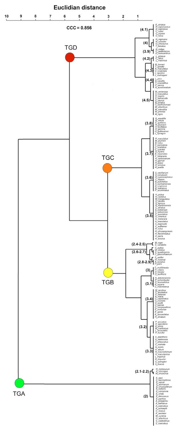
Figure 3 Cluster analysis of the coral reef fish community of the eastern coast of the Yucatán Peninsula, using the trophic index as grouping factor and Euclidian distance. In parenthesis, the trophic values of each cluster. CCC: cophenetic correlation coefficient. Trophic groups: A, green dot; B, yellow dot; C, orange dot; D, red dot.
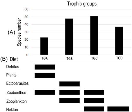
Figure 4 Comparative bar chart of the (A) number of species per trophic group, and (B) diet categories per trophic group. TG: trophic group.
The morphological variation of the community is mainly related to the size of the eyes, the position of the mouth, the size of the dorsal and anal fins, and the deep or elongation of the body (Fig. 5). The first PC summarized 37% of the variation and segregated species with small eyes, posterior dorsal and anal fins, terminal mouth, and short caudal peduncle (e.g., Diodon hystrix; PC1+); from species with elongated dorsal and anal fins and superior mouth (e.g., Bothus lunatus; PC1-). The second PC summarized 58% of the variation and segregated elongated species, with superior mouth and small eyes (e.g., Sphyraena barracuda; PC2+), from deep-bodied species, with large eyes and terminal mouth (e.g., Aluterus schoepfii; PC2-).
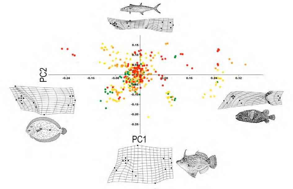
Figure 5 Principal component analysis of the morphometric variation among all species, using PC1 and PC2. Deformation grids indicate extreme shape along PC axes. An illustration was added to exemplify the fish species that each deformation grid represents. Trophic groups: A, green dot; B, yellow dot; C, orange dot; D, red dot.
Morphological variation was observed but there was overlap between all trophic groups (Fig. 6). The morphological variation showed how species in trophic group a have small eyes and mouth and the eyes are relatively backward from the mouth; the eyes and mouth are larger in group c, which includes highly elongated species (e.g., functional group c3) and deep-bodied species (e.g., functional group c5); trophic group b has deep-bodied species with mean sized eyes and mouth; and finally trophic group d includes the species with the larger mouths and the eyes positioned over the mouth (Fig. 6).
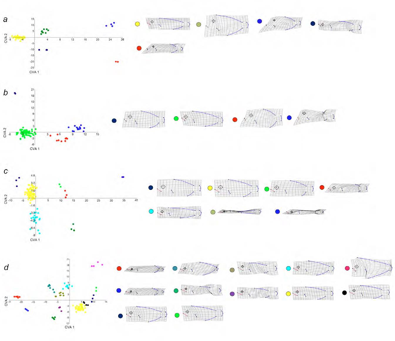
Figure 6 Canonical variables analyses of trophic groups showing the resultant functional groups and their morphological variation. CVAa: a1, red circles; a2, blue circles; a3, navy blue circles; a4, green circles; a5, yellow circles. CVAb: b1, red circles; b2, blue circles; b3, navy blue circles; b4, green circles. CVAc: c1, red circles; c2, blue circles; c3, dark green circles; c4 green circles; c5, navy blue circles; c6, aqua circles; c7 yellow circles. CVAd: d1, red circles; d2, blue circles; d3, pink circles; d4, dark green circles; d5, purple circles; d6, green circles; d7, navy blue circles; d8, aqua circles; d9, brown circles; d10, grey circles; d11, black circles; d12, yellow circles. In the morphological grids (right) marked in black the eye, in red the snout, and in blue the base of the dorsal fin, caudal fin, anal fin, and pectoral fin.
However, Manova results showed significant differences in morphology between the trophic groups (Wilks’ lambda = 0.36; F = 4.73 84-985; p = 9.86E-34; Pillai trace = 082; F = 4.47 84-993; p = 4.388E-31). By the analyses of shape per trophic group, we found 28 functional groups (Table 2). The trophic group d was the most diverse with 12 functional groups (Wilks’ lambda = 3.375E-11; F = 20.24 308-658; p = 1.435E-213; Pillai trace = 8.429; F = 8.315 308-781; p = 5.048E-126; Fig. 6d), followed by trophic group c with 7 functional groups (Wilks’ lambda = 4.429E-05; F = 10.14 168-379; p = 1.217E-76; Pillai trace = 4.301; F = 6.15 168-408; p = 8.925E-51; Fig. 6c), trophic group a with 5 functional groups (Wilks’ lambda = 9.277E-07; F = 25.79 112-90; p = 5.4971E-41; Pillai trace = 3.841; F = 21.59 112-1110; p = 2.809E-41; Fig. 6a), and trophic group b with 4 functional groups (Wilks’ lambda = 0.0007073; F = 29.82 84-243; p = 1.10E-41; Pillai trace = 2.683; F = 25.1 84-249; p = 3.85E-85; Fig. 6b).
Functional group c7 is the richest with 34 species, followed by b4 with 33 species, d12 with 18 species, a5 with 17 species and c6 with 10 species, while 13 groups are monospecific (a1, a2, a3, b3, c1, c2, c3, c4, c5, d2, d3, d5, d6, and d10). Seven functional groups were distributed in all localities (a4, a5, b4, c6, c7, d7, d12), 3 were absent only in 1 locality (b1, c1, d10), and 8 were present in only 1 locality (a2 in Xahuayxol; a3 in Mahahual; b3 in Boca Paila; c4 in Tampalam; c5 in Mahahual; d1 in Mahahual; d3 in Xkalak; d5 in Yuyum-Xamach).
A database with 5 variables (coral cover, number of reef zones, protection of the reserve, coded as 1 inside the reserve and 0 outside the reserve, number of species, and number of functional groups per locality; Table 1) was analyzed to determine the effect of habitat complexity and the protection of the Sian-Ka'an Biosphere on the fish and functional diversity. Regression analyses results showed relationships among most variables, except with the variable protection of the Sian-Ka'an Biosphere Reserve. The variables with the strongest relationship were coral cover, number of reef zones, and number of fish species per locality (Table 3).
Table 3 Regression analysis on the relation of habitat complexity and protection of the Sian-Ka’an Biosphere Reserve on the coral reef fish community. NFS: number of fish species; NFG: number of functional groups; S-KBR: protection of the Sian-Ka’an Biosphere Reserve; NRZ: number of reef zones; CC: coral cover. Standard error (se). Statistically significant relationships between variables are highlighted in bold.
| NFG | S-KBR | NRZ | CC | ||
| NFS | r2 | 0.5475 | 0.1782 | 0.7896 | 0.8106 |
| se | 1.7489 | 11.019 | 3.0150 | 0.1652 | |
| t | 3.2998 | 1.3969 | 5.8124 | 6.2065 | |
| p | 0.0046 | 0.098 | 0.0001 | 0.0001 | |
| CC | r2 | 0.3001 | 0.2453 | 0.8541 | |
| se | 1.905 | 9.2705 | 2.2011 | ||
| t | 1.822 | 1.7105 | 7.2596 | ||
| p | 0.0487 | 0.0607 | 0.0000 | ||
| NRZ | r2 | 0.2533 | 0.2143 | ||
| se | 0.1141 | 0.5571 | |||
| t | 1.7475 | 1.5667 | |||
| p | 0.0537 | 0.0758 | |||
| S-KBR | r2 | 0.0211 | |||
| se | 0.0705 | ||||
| t | 0.4401 | ||||
| p | 0.3351 |
Discussion
Our results on the coral reef fish community of the eastern coast of the Yucatán Peninsula, belonging to the North Sector of MBRS indicate that variation in habitat complexity was a significant factor explaining fish and functional diversity. Accordingly, a highly complex habitat may support more potential niches and a greater range of trophic groups favoring morphological radiation in its inhabitants and therefore a functionally diverse suite of fauna (Aguilar-Medrano et al., 2012; Arias-González et al., 2011; Fulton, 2007; Klopfer & MacArthur, 1961; Palumbi, 1997).
The Caribbean is one of the 5 world hotspots for marine biodiversity (Rivera-Monroy et al., 2004) and according to our study, a functionally diversified environment. However, resilience depends on many more variables, which allow an ecosystem to resist perturbations and recover (Folke et al., 2004). According to our results, the Caribbean might not be a highly resilient ecosystem because the functional groups show low redundancy (from the 28 functional groups, 22 include 1 to 5 species) and the reef fish community strongly depends on the coral cover. Besides this, the Caribbean had few hard barriers to dispersal, behaving as a single ecosystem, and thus imposing little buffering from biological or physical disturbance (Roff & Mumby, 2012). Thus, in the case of large-scale disturbance, this area might be hardly affected. As has been shown in different studies, the Caribbean Sea is one of the regions where the most serious declines in terms of reef area, health, and fisheries productivity is occurring (Alvarez-Filip et al., 2009; Gardner et al., 2003; Miloslavich & Klein, 2005; Perry et al., 2013).
As found in previous analyses, our results show that habitat complexity is highly related to fish diversity and functional diversity in the Caribbean reefs (Alvarez-Filip et al., 2009; Arias-González et al., 2008; Núñez-Lara & Arias-González, 1998). This is observed clearly when comparing Yuyum-Xamach or Mahahual, the localities with most of the highest values of coral cover, fish diversity, and functional diversity with the presence of specific functional groups for each locality, against Puerto Morelos, the locality with the lowest values, which only presents the common functional groups, i.e., those present in all localities.
On the other hand, from the 8 localities with 4 reef zones, in 6 of those, the slope is the zone with the highest fish diversity, while in all localities the lagoon is the zone with the lowest fish diversity. Cinner et al. (2016) proposed a new approach to characterize and manage reefs through the classification of reef zones based on environmental and socioeconomic variables. Accordingly, a bright spot is a zone where the ecosystem is substantially better and a dark spot is a zone where ecosystems are worse. In this sense, according to our results, the slope is a bright spot in all studied localities, without distinguishing between localities inside or outside the reserve. The presence of these bright spots in all studied localities produces a belt of diversity, favoring connectivity. Thus, conservation of these bright spots can ensure the recovery of areas where pressures have produced loss of habitat complexity and diversity.
According to our results, the protection of the Sian-Ka'an Biosphere Reserve does not show a relationship with any of the response variables. Studies on the effect of the marine reserves on fish communities indicate that it is possible to observe results of protection after a few years (Claudet et al., 2006; Halpern & Warner, 2002; Russ et al., 2005) or decades (Claudet et al., 2008; Halpern, 2003; McClanahan & Arthur, 2001; Micheli et al., 2004). Because our data date from 13 and 14 years after the declaration of the marine reserve, time could be a reason for our result and would be useful for testing whether the factors identified here remain important over a longer period.
There is evidence indicating that marine reserves cannot protect reefs from large-scale pollution or global warming (Allison et al., 1998; Hughes et al., 2003; Jameson et al., 2002; Jones et al., 2004). The declaration of marine reserves is gaining importance as a way to protect marine life and avoid anthropogenic impacts, which represents a steppingstone in the protection of these ecosystems. However, despite its popularity, decisions on the design and location have largely been the result of political processes, giving little importance to biological considerations (Agardy, 1994; Halpern, 2003; Jones et al., 1992; McNeill, 1994). Therefore, it is important to reconsider the way we enact and manage marine reserves, including functional approaches that allow us to understand the interactions in the ecosystem, how disturbances affect the structure and function of reefs and permit us to detect key variables to monitor and manage these ecosystems (Bellwood et al., 2004; Hughes et al., 2003).
It is generally accepted that diversity enhances stability in multitrophic systems (Steiner et al., 2005). Our results indicate that the Mexican Caribbean hosts a relatively high diverse conglomerate of fish. However, a community highly dependent on habitat complexity, even with a high functional diversity but low redundancy, as is the case of our study, has the risk of losing functions due to disturbance (Paddack et al., 2009). Functional groups analysis allowed us to have a better idea of how the system works, understanding the trophic and functional divisions and by monitoring, detect early changes in the ecosystem.
If we know that coral reefs support over a quarter of the world’s small-scale fisheries, generate jobs, provide for many of the 275 million people living close by, and provide critical sea defenses against storms, flooding, and land erosion (Spalding & Brown, 2015), still the pressures over these environments are high. In consequence, it is crucial to develop a better governance by taking efficient actions that regulate the use and management of these ecosystems.
According to our results, we recommend the following measures to protect and manage the ecosystem: 1) increase efforts in the monitoring of fragile functional groups (locality-specific functional groups) and species-specific functional groups. These groups depend on highly specific niches, thus in the case of disturbance, they might be the first to disappear. Also, increase efforts in the monitoring of functional groups belonging to the trophic group a, which feed mainly on detritus and algae, because their biomass can increase due to coral-algae reefs shift phases and/or increases in human drainage discharges to the ocean; 2) recognize the slope zone in the Caribbean as a bright zone and accordingly, regulate its use. According to our results, this zone acts as a corridor of diversity for the whole area; 3) compare the functional groups year by year in order to detect early changes in the ecosystem and determine the direction of the change, and 4) educate the fishing community and public in conservation.

