


 nova página do texto(beta)
 Inglês (pdf)
 Artigo em XML
 Referências do artigo
 Enviar este artigo por email
 Citado por SciELO
  Similares em
SciELO
Similares em
SciELO 
 Permalink
Introduction
Spiders inhabit almost all terrestrial ecosystems and are particularly diverse in the tropical and subtropical regions where most of the new species are expected to be found (Foelix, 2011). At the present there are more than 45,862 described species and Araneomorphae accounts for 93% of the total (WSC, 2016). It is estimated by taxonomic comparisons that between 2 and 5 times more species could be extant (Adis & Harvey, 2001; Coddington & Levi, 1991; Coddington, Giribet, Harvey, Prendini, & Walter, 2004; Platnick, 1999). Field data of 5 inventories from tropical forests worldwide averaged 274 species collected per ha, estimating an average richness of 403, with 812 species as the highest estimation from a Rainforest in Peru (Coddington, Agnarsson, Miller, Kuntner, & Hormiga 2009; Coddington, Griswold, Silva-Dávila, Peñaranda, & Larcher, 1991; Miller & Pham, 2011; Silva & Coddington, 1996; Sørensen, Coddington, & Scharff, 2002). Also the beta diversity is higher in tropical regions, a comparison between 2 spider inventories in Peru and Bolivia estimated only 5-20% shared species at similar elevation and 0.8-2.8% between elevations (Agnarsson, Coddington, & Kuntner, 2013). However, many more inventories would be required to estimate spider diversity and observe worldwide patterns using field data, therefore the taxonomic comparisons are our best estimate so far.
Faunistic inventories with spiders, as with other megadiverse taxa, present 2 main challenges: first, it is virtually impossible to collect all species in a particular area, and second, the large amount of time invested in the identification of specimens for taxonomically poorly documented and megadiverse taxa. Species richness estimators have been developed to address the first problem by extrapolating rarefaction curves, using species abundance distributions and non-parametric estimators that combine accumulation curves with the proportion of rare species in the sample (Colwell & Coddington, 1994; Colwell et al., 2012; Gotelli & Colwell, 2001). Also addressing this problem a pivotal advance happened for spiders when a standardized sampling protocol was proposed by Coddington et al. (1991) which combines several uniform techniques. This protocol has been used by several studies worldwide, incorporating more collecting techniques and new species richness estimators (Cardoso, 2009; Cardoso, Scharff, et al., 2008; Cardoso, Gaspar, et al., 2008; Coddington, Young, & Coyle, 1996; Coddington et al., 2009; Dobyns, 1997; Höfer & Brescovit, 2001; Miller & Pham, 2011; Scharff, Coddington, Griswold, Hormiga, & Bjørn, 2003; Sørensen, 2003; Toti, Coyle, & Miller, 2000).
The second problem has been addressed only recently, and although the taxonomic challenge of identifying species for poorly documented megadiverse taxa remains huge, considerable progress has been made thanks to the advances in digital imaging technology used to comprehensively document morphology, decreasing costs of DNA sequencing and web resources to share this information worldwide (Wheeler, 2008; Wilson, 2004). This new approach has been named cyberdiversity and has been proposed as a solution to the taxonomic impediment (Miller, Miller, Pham, & Beentjes, 2014). Some recent faunistic spider inventories have been pioneers in making available on the internet extensive image databases of all morphospecies (Ramírez, 2004), combining such databases with taxonomic descriptions for particular taxa (Miller, Griswold, & Yin, 2009) or providiong morpholocial data, DNA barcodes (www.digitalspiders.org) and evaluating how biodiversity changes in function of space, climate or other environmental variables (Miller et al., 2014).
Mexico is considered the world's fifth most diverse country (Llorente-Bousquets & Ocegueda, 2008). This diversity is product of the convergence of the Nearctic and Neotropical biotas combined with a rough topography defined as the Mexican Transition Zone (Espinosa-Organista, Ocegueda-Cruz, Aguilar-Zúñiga, Flores-Villela, & Llorente-Bousquets, 2008). The first description of a mexican spider was done by Lucas (1833), since then, most of the taxonomic work of the Mexican araneofauna has been done mainly by European and American arachnologists: Becker (1878, 1886), Koch (1836,1847), Peckham and Peckham (1883, 1909), Simon (1884, 1909), Gertsch (1933), Muma and Gertsch (1964), Levi (1953, 2005), Platnick (1972), and Bolzern, Platnick, and Berniker (2015). These authors published approximately 150 taxonomic works since then for the Mexican fauna (WSC, 2016); the references mentioned above include the first and last relevant papers on this topic. The most important taxonomic studies with spiders in the country are more than a century old and still useful references for this fauna (Cambridge, 1889, 1897; Keyserling, 1880, 1893).
The first spider catalog for Mexico reported 1,598 species (Hoffman, 1976). Since then 3 catalogs have been published reporting approximately 2,300 species (Francke, 2013; Jiménez, 1996; Jiménez & Ibarra-Núñez, 2008). According to data extracted from the World Spider Catalog (2016) there are currently 2,159 described species in 69 families occurring in Mexico representing ca. 4.7% of the world spider fauna.
A search in Web of Science v. 5.21 using the keywords Araneae or spider and biodiversity or faunistic, gave 263 results worldwide of which at least 18 are focused in the diversity of Araneae species for Mexico. In the last 24 years there have been several faunistic studies on the Mexican araneofauna restricted to a group or guild (Arana-Gamboa, Pinkus-Rendón, & Rebollar-Téllez, 2014; Bizuet-Flores, Jiménez-Jiménez, Zavala-Hurtado, & Corcuera, 2015; Corcuera, Valverde, Zavala-Hurtado, de la Rosa, & Duran-Barrón, 2010; Corcuera et al., 2015; Jiménez & Navarrete, 2010; Méndez-Castro & Rao, 2014), focuses on synantropic species (Desales-Lara, Francke, & Sánchez-Nava, 2013; Rodríguez-Rodríguez, Solís-Catalán, & Valdez-Mondragón, 2015; Salazar-Olivo & Solís-Rojas, 2015), or have an agroecological view (Ibarra-Núñez & García-Ballinas, 1998; Lucio-Palacio & Ibarra-Núñez, 2015; Marín & Perfecto, 2013). Studies that represented most of the spider diversity that inhabits a certain area by using a mixture of methods provide valuable information regarding ecological comparisons and species lists (Gómez-Rodríguez & Salazar-Olivo, 2012; Ibarra-Núñez, Maya-Morales, & Chame-Vázquez, 2011; Jiménez, 1991; Jiménez, Nieto-Castañeda, Correa-Ramírez, & Palacios-Cardiel, 2015; Maya-Morales, Ibarra-Núñez, León-Cortés, & Infante, 2012; Pinkus-Rendón, León-Cortés, & Ibarra-Núñez, 2006). However, comparisons with most of these studies are difficult because they used different collecting protocols, sample effort units and plot areas; regardless than standardized protocols for the group had been proposed and applied worldwide (Coddington et al., 1991, 1996, 2009; Dobyns, 1997; Scharff et al., 2003; Silva & Coddington, 1996; Sørensen et al., 2002; Toti et al., 2000). Furthermore this protocol is flexible enough to evaluate and incorporate other environmental variables and collecting techniques; the only requirements are specifying the area of the plot and using comparable sampling effort units (Cardoso, 2009; Cardoso, Gaspar, et al., 2008; Coddington et al., 2009; Ibarra-Núñez, Maya-Morales, & Chame-Vázquez, 2011; Maya-Morales et al., 2012).
Taxonomic comparisons between the Mexican inventories that included a list of the species collected obtained an average of 52% identified species. This represents a problem for direct comparisons, in particular for the unidentified morphospecies and the ones that remain as “circa” or “affinis”. Three alternatives exist for comparing unidentified taxa: wait until the new taxa are described, visit the collections where the specimens are deposited or illustrate all morphospecies with digital images available online.
The first 2 solutions have the disadvantage of waiting until formal descriptions are produced and the time and resources required for visiting the collections. The third solution makes these data immediately available and free for the scientific community or any institution with special interest in it. It also expedites the species identification process, provide identification voucher specimens and allow direct comparisons with other inventories for unidentified morphospecies that are otherwise difficult to reconcile with other studies or remain uninformative.
This last solution has never been implemented in México therefore the objectives of this paper are: to create an online image database documenting all morphospecies and species of the studied locality linked to their diversity data in the context of the new taxonomy (Wheeler, 2008), to estimate the species richness using nonparametric estimators and to analyze the impact of seasonality on the species composition.
Materials and methods
The study was conducted in the municipality of Xilitla, San Luis Potosí. This zone is part of the Sierra Madre Oriental having an altitude ranging from 600 to 2,000 m a.s.l. It is characterized by tropical vegetation; nonetheless almost half of the municipality vegetation has been transformed for agricultural use (Inegi, 2014). Spiders were collected in a 1 ha plot with homogeneous vegetation located approximately 2 km north of Xilitla (21°23′50″ N, 98°59′38″ W) inside the “Jardín Escultórico Edward James”. This site has a relatively well preserved area of 30 ha of tropical vegetation that is used primarily for ecotouristic activities.
Sampling was carried out by 6 collectors during 4 expeditions (4 days each) from August, 2011 to June, 2012. The dates for these field trips were: August 27-31, 2011; November 14-18, 2011; March 23-30, 2012; and June 10-15, 2012. Approximately 120 samples were obtained per expedition using 6 methods: looking up, looking down, cryptic, beating, Berlese funnels and pitfall traps (Cardoso, 2009; Coddington et al., 1991; Miller et al., 2014; Scharff et al., 2003; Sørensen et al., 2002; Toti et al., 2000) allocating more effort for direct methods at night following both our experience and specialized literature suggestions. Direct methods included looking up, looking down, cryptic and beating, the first 2 were implemented during night, while the other 2 were done during the day. Samples of these methods were taken randomly inside the plot taking as effort unit 1hour per sample ranging from 20 to 30 samples of each method per expedition. Non-direct methods included sifted leaf litter processed with a Berlese funnel and pitfall traps. These were implemented as follows: funnel extraction consisted of 12 samples -1.5 l each - of sifted leaf litter per expedition. Samples were processed in 12 Berlese funnels for 3 days under a 60 W light bulb. Finally 31 pitfall traps per expedition were placed randomly inside the plot.
Each sample was labeled with expedition code, collector, method, and replicate number and preserved in 96% ethanol. Adult specimens are important because only the genital features are reliable to identify species or sort different morphospecies. In most tropical inventories juvenile spiders are not identified because these faunas are so little known that attempting to identify immature specimens using morphology will result in errors produced by associating immature and adults that are not conspecific or splitting the same morphospecies in more than 1. In many cases, even adult specimens may be impossible to identify (Coddington et al., 1996, 2009; Miller & Pham, 2011; Scharff et al., 2003; Sørensen et al., 2002; Toti et al., 2000). A solution to this problem not implemented here is the use of DNA barcodes to associate immatures and adults without ambiguity (Barret & Hebert, 2005; Prendini, 2005; Raso, Sint, Rief, Kaufmann, & Traugot, 2014; Slovik & Blagoev, 2012). Adult specimens were sorted to morphospecies and determined to genus and family using the Ubick, Paquin, Cushing, and Roth (2005) and Jocque and Dippenaar-Schoeman (2006) identification keys, and several papers provided by various internet sources (BHL, 2014; among other resources). Specimens and samples were organized using Microsoft Excel and this databse is available at www.unamfcaracnolab.com/WPGS_XIL/Xilitla.html.
Digital images where done with the following microscopes and digital cameras: Leica MZ16A, Nikon SMZ1000 for external morphology and Leica DM4000M for internal genital anatomy. Digital cameras were a Leica DFC500 and a Nikon DS-U2 for external anatomy and Nikon DXM1200 digital for structure of internal genitalia. The female internal genitalia were digested using pancreatin (Álvarez-Padilla & Hormiga, 2007), cleared using clove oil and mounted in semipermanent preparations (Coddington, 1983). Voucher specimens are deposited at the Laboratorio de Aracnología, Facultad de Ciencias, Universidad Nacional Autónoma de México and the California Academy of Sciences. Images for each morphospecies included approximately 15 standard views that covered most of their somatic and genital anatomy. An average 20 digital images were taken by standard view and combined with the program Helicon Focus 5.3 using the default values except radius set up at 44 and smoothing setup at 1. Rendering Method A was used for external anatomy and rendering Method B for cleared genitals. In some cases levels and contrast of the images were modified using Adobe Photoshop CS2 version 9.0. A selection of 2,238 images for all morphospecies is available online at www.unamfcaracnolab.com (Álvarez-Padilla Laboratory, 2014). Several arachnologists contributed with the species and genus identification speeding up the process, they are included in the Acknowledgements section and referenced with their respective identification on the website.
Species richness nonparametric estimation and the similarity analysis between seasons were performed with the program EstimateS 9.1.0 (Colwell, 2013). This program includes abundance based (Chao 1 and ACE), incidence based estimators (Chao 2, ICE, both Jacknifes and bootstrap). To asses if there were differences between the seasonality and the species collected at each expedition. Also the Shannon-Wiener diversity index was obtained for each of the expeditions and compared pair wise using the Hutcheson T-test (Hutcheson, 1970).
Results
A total of 485 samples were obtained from which 86 were beating, 45 berlese, 89 criptic, 82 looking down, 87 looking up and 96 pitfall traps capturing 10,661 spiders of which 4,118 were adults (38.6% of the total) representing 205 species and 39 families (Appendix 1). Almost 56% of the species found remained unidentified and many of these are expected to be new. Taxonomic identifications included 91 morphospecies identified to species level, 12 as confer or similar to a described species, 86 identified to genus and 16 only to family level. Each species was documented with an average of 15 images when both sexes were found and 8 images when only 1 sex was available. These standard views were: cephalotorax anterior view, habitus dorsal, lateral and ventral views for both sexes (total 8 images), 4 views on average to document male genital anatomy and three images for the female genitalia. Species richness estimations based on abundance data gave between 256 species with ACE and 290 with Chao 1; of these 2 estimations only Chao 1 calculates 95% confidence intervals that varied between 246 and 376. Incidence based estimations obtained 280 species with Chao 2, ICE 253, 229 bootstrap and 260 and 295 with Jacknife 1 and 2, respectively. Only Chao 2 computes confidence intervals that ranged between 242 and 356 species. A total of 55 species were singletons and 18 doubletons, 55 species were also represented only once in a sample (uniques) and 20 represented in only 2 samples (duplicates). The highest species estimation was given by Jackknife 2 with 294 species and the lowest with 229 was given by bootstrap (Table 1). The species accumulation curves exhibit stable behavior after the 100 samples but do not present a clear asymptote, likewise the singleton and doubleton curves did not intersect, an observation consistent with the proportion of rare species (Fig. 1).
Table 1 Observed and estimated species richness.
| Species | SD | |
|---|---|---|
| Samples | 485 | |
| Individuals | 4120 | |
| Observed richness | 205 | |
| Singletons | 55 | - |
| Doubletons | 18 | - |
| Uniques | 55 | - |
| Duplicates | 20 | - |
| ACE | 255.85 | 0 |
| ICE | 253.3 | 0 |
| Chao 1 | 289.01 | 31.45 |
| Chao 1 95% CI lower bound | 246.31 | - |
| Chao 1 95% CI upper bound | 375.86 | - |
| Chao 2 | 280.47 | 27.83 |
| Chao 2 95% CI lower bound | 242.48 | - |
| Chao 2 95% CI upper bound | 356.95 | - |
| Jack 1 | 259.89 | 9.2 |
| Jack 2 | 294.78 | 0 |
| Bootstrap | 229.03 | 0 |
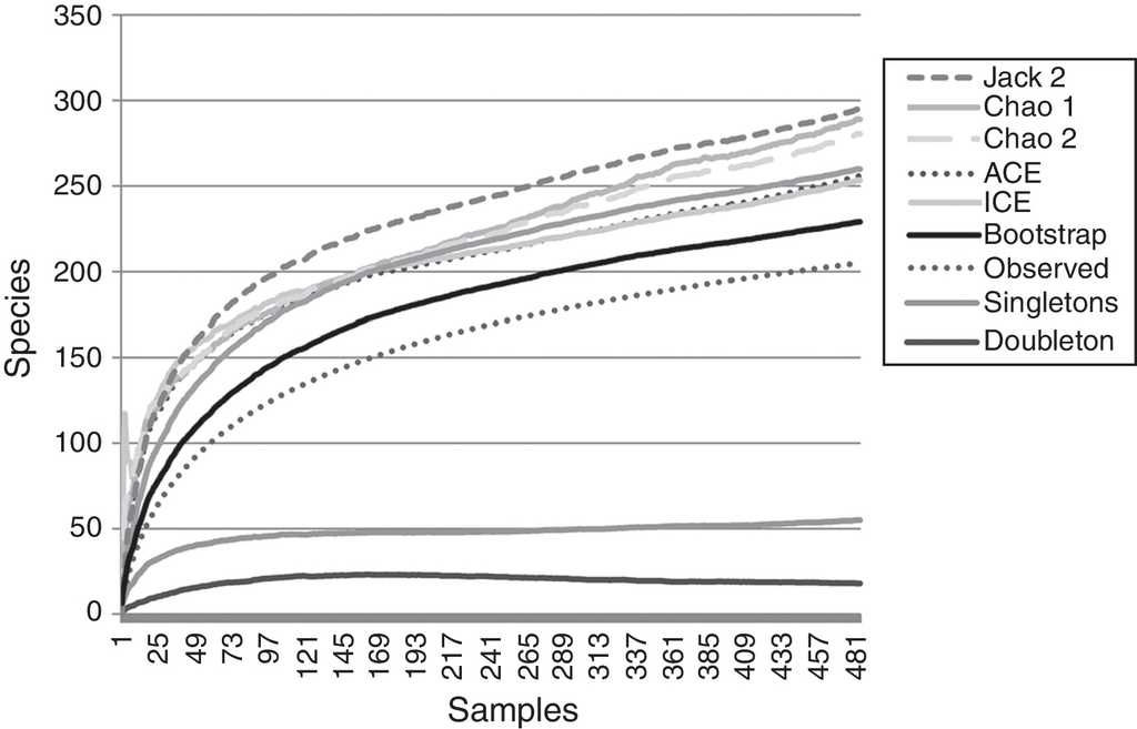
Figure 1 Species accumulation and estimation curves. Data only includes adult specimens collected in 1hectare plot. Six non-parametric estimators based on: abundance (Chao 1, ACE), incidence (Chao 2, ICE) and resampling (Jackknife 2, Bootstrap) included. Singletons and doubletons are also graphed.
Comparisons between the species lists in relation to seasonality obtained that the expeditions of March and June were the richest with 136 and 135 species, respectively sharing 87; followed by November with 106 and August with 88 species sharing 57. Shannon-Wiener diversity index per expedition were August 3.38; November 3.75; March 3.72 and June 4.03. Pair wise differences between these expeditons were evaluated using a Hutchenson t-test showing that only March and November expeditions (t (1998.6) 0.41 < p = 1.64) were significantly different between them. Most rare species were found in March and June with 23 and 17 singletons, respectively; whereas August and November had 7 and 8 singletons.
An average of 10.2 (±15.5) adult specimens per species were collected. Twenty were represented by 50 or more specimens, of these taxa Theridion sp. 1 (Theridiidae) (457) was the most abundant followed by Pirata pagicola Chamberlin, 1925 (290) (Lycosidae), Thymoites illudens Gertsch and Mulaik, 1936 (266) (Theridiidae) and Phrurolithidae sp. 1 (185); the abundance for the other 16 species ranged between 54 and 179 specimens (Fig. 2). The 185 taxa not included in this plot were represented by an average of 7.4 (±9.1) specimens per species including the singletons and doubletons mentioned above.
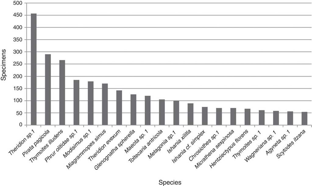
Figure 2 Histogram of the twenty more abundant species. Data includes abundance of all adult specimens per species collected in the inventory.
The most abundant family was also Theridiidae with 1,432 specimens, followed by Pholcidae (304) and Lycosidae (295). Four families were represented only by 1 specimen (Agelenidae, Hahniidae, Philodromidae and Zorocratidae). Theridiidae was the richest family with 51 species representing 25% of the total followed by Salticidae and Araneidae with 25 each accounting together for the 23.1%. Thirteen families were represented only by 1 species (Appendix 1).
Discussion
More than 55% of the species collected in this inventoy remained as unidentified and are likely new. Some of these species were identified as related to a described species (aff. or cf.) indicating in the website the characteristics that are different between them. Whereas other species were only identified to genus and in some cases to family level (sp.) depending on the taxonomic problems particular of each taxon. The percentage of new species in relation to the total of species collected was compared in 14 studies that did not necessarily follow Coddington et al. (1991) protocol, but included a species list. Results ranged between 0 and 13.09% of unidentified species for temperate regions. In contrast, the percentage of unidentified taxa for tropical regions varies between 49.18 and 100% with an average of 43.6% unidentified taxa (Table 3).
Table 3 Percentages of undetermined species in spider inventories.
| Author | Undet. spp. | Geographic area |
|---|---|---|
| Dobyns (1997) | 0.00% | Ellicott Rock, USA |
| Scharff et al. (2003) | 0.00% | Hestehaven, Denmark |
| Toti et al. (2000) | 5.46% | Great Smoky Mountains, USA |
| Coddington et al. (1996) | 5.68% | Ellicott Rock, USA |
| Cardoso, Gasper, et al. (2008) | 13.09% | Mata da Albergaria, Portugal |
| Höfer and Brescovit (2001) | 48.91% | Reserva Ducke, Brazil |
| Ricetti and Bonaldo (2008) | 49.18% | Serra do Cachimbo, Brazil |
| This study | 56.03% | Xilitla, Mexico |
| Ibarra-Núñez et al. (2011) | 64.47% | Volcán Tacaná, Mexico |
| Raizer et al. (2005) | 65.53% | Bacia do Rio Paraguai, Brazil |
| Bonaldo and Dias (2010) | 88.86% | Porto Urucu, Brazil |
| Sørensen et al. (2002) | 95.75% | Uzungua Mountains, Tanzania |
| Silva and Coddington (1996) | 100.00% | Pakitza, Peru |
When comparisons are attempted between published inventories the biggest problem is the high percentage of species that are either unidentified or the identification is doubtful, particularly for tropical regions with megadiverse taxa that are poorly documented. The tool provided by cyberdiversity (Miller et al., 2014) that directly address this problem is the publication of extensive image databases available on the internet coordinated with faunistic inventories. These databases allow direct comparisons of morphospecies that remain unidentified either because they are new or because the taxonomy of the group needs a thorough revision. In addition, these databases also provide voucher specimens that give evidence of the accuracy of the taxonomic determinations, illustrate interspecific geographic variations and expedite the process of new species recognition.
It has been estimated that 1 hectare of tropical forest may support between 300 and 800 species of spiders (Coddington et al., 1991, 2009). The present study reports a total of 205 species for a remnant of tropical forest. Similar studies done in Mexican territory have obtained similar richness ranging from 112 to 243 species (Bizuet-Flores et al., 2015; Jiménez et al., 2015; Maya-Morales et al., 2012). Inventories conducted in tropical areas of South America ranged between 121 and 352 species (Coddington et al., 2009; Nogueira, Pinto-da Rocha, & Brescovit, 2006; Raizer, Hilton, Indicatti, & Brescovit, 2005; Ricetti & Bonaldo, 2008; Silva & Coddington, 1996; Yanoviak, Kragh, & Nadkarni, 2003). For temperate ecosystems 123.5 (±51.1) species were collected, the highest richness was observed in a Quercus spp. forest in Portugal with 204, and the lowest in a scrubland in USA with 60 species (Cardoso, Scharff et al., 2008, Toti et al., 2000). Eighteen of these spider inventories worldwide that use comparable sampling protocols were analyzed collecting 211.1 (±SD 138.69) species (Table 2).
Table 2 Abundance, richness and estimated number of species of 18 spider inventories worldwide.
| Vegetation | Abundance | Richness | Estimation | Estimation | Estimation | Study |
|---|---|---|---|---|---|---|
| (range) | mean | SD | ||||
| Coastal forest | 8,710 | 66 | 74-88 | 81 | 7 | Scharff et al. (2003) |
| Grassland | 1,853 | 91 | 106-159 | 131.75 | 22.88 | Toti et al. (2000) |
| Hardwood forest | 1,629 | 89 | 117-128 | 122.67 | 5.51 | Coddington et al. (1996) |
| Montane forest | 5,233 | 149 | 165-201 | 183 | 18 | Sørensen (2003) |
| Montane forest | 9,096 | 170 | 183-215 | 195 | 6.93 | Sørensen et al. (2002) |
| Pantanal | 602 | 206 | 299 | 299 | 34 | Raizer et al. (2005) |
| Quercus forest | 10,808 | 204 | 232-260 | 242.75 | 12.84 | Cardoso, Gaspar, et al. (2008) |
| Quercus forest | 7,423 | 168 | 188-214 | 199 | 11.6 | Cardoso, Henriques, et al. (2008) |
| Scrubland | 3,059 | 115 | 116-192 | 160.11 | 22.83 | Cardoso, Scharff, et al. (2008) |
| Scrubland | 573 | 60 | 68-97 | 75.75 | 14.38 | Toti et al. (2000) |
| Tropical forest | 5,965 | 352 | 443 | - | - | Coddington et al. (2009) |
| Tropical forest | 3,912 | 506 | - | - | - | Höfer and Brescovit (2001) |
| Tropical forest | 1,208 | 112 | 123-138 | 132.8 | 5.81 | Maya-Morales et al. (2012) |
| Tropical forest | 2,010 | 262 | 336-385 | 360.5 | 34.65 | Miller and Pham (2011) |
| Tropical forest | 3,148 | 121 | - | - | - | Nogueira et al. (2006) |
| Tropical forest | 2,750 | 427 | 614 | - | - | Ricetti and Bonaldo (2008) |
| Tropical forest | 2,616 | 498 | 720-812 | 766.75 | 41.13 | Silva and Coddington (1996) |
| Tropical forest | 1,163 | 204 | - | - | - | Yanoviak et al. (2003) |
| Tropical forest | 4,121 | 212 | 237-298 | 275 | 22.44 | This study |
Non-parametric estimators show that the 205 species found in this inventory represent between the 89.5% and 69.7% of the estimated species in the sampled area. This is consistent with other tropical inventories where usually between 50% and 85% of the araneofauna is found and the estimated curves do not present a clear asymptote (Bonaldo & Dias, 2010; Coddington et al., 1996, 2009; Maya-Morales et al., 2012; Miller & Pham, 2011; Ricetti & Bonaldo, 2008; Sørensen et al., 2002). As the samples accumulate in the inventory, it is less likely to add new species to the inventory, most of which will represent either rare species of the study site or vagrant species that do not belong to the studied community (Cardoso, 2009; Coddington et al., 2009; Jiménez-Valverde & Hortal, 2003; Moreno & Halffter, 2000).
The variation of the diversity in each of the expeditions was compared using the Hutcheson test to evaluate statistically the seasonal differences in the spider community. Comparisons between the species lists in each expedition reveals March as the richest with 136 species and August as the least rich with 88 species. The relative abundance shows that March is also the month with more adult abundance (308) and November is the one with least adult representation (809). This could be correlated with the phenology of the different spiders groups during the year, independently of the collecting effort. Nevertheless it is recommended for arthropod inventories to sample at different times of the year increasing the probability of collecting adult specimens for most taxa.
As Cardoso (2009) suggests, different study sites require different number of samples per collecting method. In the case of Xilitla, the methods that covered the vegetation were the most effective, representing comprehensively the fauna they are designed for in a smaller number of samples than the methods that cover ground spiders and cryptic habitats as revealed by the steepness of the curves. Therefore, in order to increase the number of ground and wandering species, more effort should be put in these methods. These differences reflect the microhabitats where most of the spiders are found. However, the selection of collecting techniques for a given ecosystem follows their suitability; for example, collecting with sweeping nets in this forest remnant would be impossible due to the tangled vegetation. Therefore, it is important to consider that although in every inventory there are methods that are more efficient than others, covering most suitable microhabitats helps to have a better representation of the community sampled especially for rare species.

