SciELO - Scientific Electronic Library Online

 
vol.66 número2Selective Pb(II)-Imprinted Polymer for Solid Phase Extraction in the Trace Determination of Lead in Infant Formula by Capillary ElectrophoresisExperimental Study and Modeling of the Corrosion Inhibition of Mild Steel in 1M Hcl with Novel Friendly Butanolic Extract of Ephedra Major índice de autoresíndice de materiabúsqueda de artículos
Home Pagelista alfabética de revistas  

Servicios Personalizados

Revista

Articulo

Indicadores

Links relacionados

  • No hay artículos similaresSimilares en SciELO

Compartir


Journal of the Mexican Chemical Society

versión impresa ISSN 1870-249X

J. Mex. Chem. Soc vol.66 no.2 Ciudad de México abr./jun. 2022  Epub 05-Dic-2022

https://doi.org/10.29356/jmcs.v66i2.1712 

Articles

Non-Relativistic Ro-Vibrational Energies of Chlorine Molecule for Molecular Attractive Potential Model

C.A. Onate*  1 

I.B. Okon2 

M.C. Onyeaju3 

1Physics Programme, Department of Physical Sciences, Landmark University, Omu-Aran, Nigeria.

2Theoretical Physics Group, Department of Physics, University of Uyo, Nigeria.

3Theoretical Physics group, Department of Physics, University of Port Harcourt, P.M.B. 5323 Choba, Port Harcourt-Nigeria.


Abstract

We obtained the solutions of the radial Schrödinger equation with the modified molecular attractive potential model by employing the supersymmetric WKB method, and present the non-relativistic rotation-vibrational energy equation for diatomic molecules. Using the energy equation and the spectroscopic parameters of chlorine molecule, we computed the vibrational energy eigenvalues for various quantum states. The calculated results are found to be in agreement with the experimental values.

Keywords: Wave equation; eigensolutions; bound state; Schrὅdinger equation

Resumen

Obtenemos las soluciones de la ecuación radial de Schrödinger con el modelo de potencial molecular atractivo modificado empleando el método WKB supersimétrico, y presentamos la ecuación para la energía rotacional-vibracional norelativista para moléculas diatómicas. Utilizando la ecuación para la energía y los parámetros espectroscópicos de la molécula de cloro, calculamos los valores propios de las energías vibracionales para varios estados cuánticos. Se encuentra que los resultados calculados están en acuerdo con los valores experimentales.

Palabras clave: Ecuación de onda; soluciones propias; estado ligado; ecuación de Schrödinger

Introduction

Based on the usefulness of internuclear energy potential function that describes the molecular structure, there has been a radical interest devoted to the determination of energy spectrum of diatomic molecules. The potential function involves usually consists of three spectroscopic parameters. Using the spectroscopic parameters, several authors have studied different molecules under different energy potential models in terms of vibration transitional frequency and validated their results by comparing it with the experimental data [1-8]. Depending on the potential function and the molecule to be studied, some calculated results fairly agreed with the experimental values while others are in good agreement with the experimental values. In ref. [1], the authors obtained the average absolute deviation of Morse potential function for X1Σ+ of scadium monoiodide as 0.0344%. Liu et al. [5], obtained average deviation of improved Rosen-Morse potential model and the Morse potential function for 33Σg+ of cesium dimer as 0.036% of De and 0.121% of De respectively. These authors also obtained the average deviation of the same potentials for 51Δg state of sodium molecule as 0.225% of De and 0.792% of De Recently, Onate and coauthors [6], modified an attractive potential to a molecular attractive potential model and used it to study 33Σg+ state of cesium and a3Σu+ state of lithium molecules via the methodology of parametric Nikiforov-Uvarov. Their calculated results were found to agree with the experimental values. They deduced the percentage average deviation of the calculated results from the experimental values. Precisely, the percentage average deviation for cesium molecule is 0.4415% while that of lithium molecule is 0.0007%. Though the two results are in good agreement with the experimental values, the potential model fits the computation of lithium molecule compared to cesium molecule. The molecular attractive potential function is given as [6]

Ux=Deλ1e2axee-2ax+λ2eaxee-ax+λ3(1-e-ax)2 (1)

where De is the dissociation energy, xe is the internuclear separation, α is a screening parameter, λ1, λ2 and λ3 are potential parameters whose values for computation depend on the author. For molecules, the screening parameter can be determine from the given potential (1) noting that

d2Vxdx2|r=re=ke4μπec2we2. (2)

Simplifying the above equation along with potential (1) gives

α=2πcweμDe(20λ1+13λ2+8λ3)-32π4c2μ2re3αewe3h2-1re. (3)

Following the value of the screening parameter above, the potential parameters are given as λ1=λ02, λ2=2(λ0-1) and λ3=λ1+λ2-2 where -<λ0<+ Motivated by the interest in the molecular attractive potential function, the present study wants to examine the molecular attractive potential function for X1Σg+ state of Cl235 The shape of molecular attractive potential is shown in Fig. 1:

Fig. 1 Molecular attractive potential model for Cl2

Bound State Solutions

The Schrὅdinger equation for a quantum system with a non-relativistic energy E and an interacting potential V(r,θ,φ) coupled with a reduced mass μ is given by

-22μ1r2rr2r+1r2sinθθsinθθ+1r2sin2θ2ϕ2-E+Vr,θ,φψr,θ,φ=0. (4)

Where is the reduced Planck’s constant and ψr,θ,φ is the total wave function. Putting the wave function in the form ψr,θ,φ=Rv,jrYj,mθ,φ, where Yj,m(θ,φ) is the spherical harmonic function, and consider the Schrὅdinger equation with (j+1)r2, the radial part of Eq. (4) becomes

-22μd2dr2+Vr-E+22μjj+1r2-Rv,jr=0, (5)

where v is the vibrational quantum number and j is the rotational quantum number. In order to obtain the analytical solutions of Eq. (5) for any arbitrary j - state, one must approximate the centrifugal term when α<<1 Several approximation schemes were developed to deal with the centrifugal term [9, 10]. In this study, we employ an improved Greene-Aldrich approximation scheme [11] to get rid of the centrifugal term.

1r2α2c0+e-αr1-e-αr2. (6)

The constant in Eq. (6) is a dimensionless constant with numerical value as 1/12 that is obtained using the following power series

α2c0+e-αr1-e-αr2=α2c0+1(ar)2-112+ar2240-ar46048+0(ar)6. (7)

If the constant c0=0 then, Eq. (6) reduces to the conventional Greene-Aldrich approximation scheme. Plugging Eq. (1) and Eq. (6) into Eq. (5), we have the following second-order Schrὅdinger-like equation of the form

d2Rv,j(r)dr2=E¯T+2μλ3De2+2μλ2Deeαre2+jj+1α2+2μλ1Dee-2αr21-e-αr2Rv,jr. (8)

where we have used the following for mathematical simplicity

E¯T=jj+1c0α2-2μEv,j2. (9)

Having obtained Eq. (8), we now employ the basic concept and formalism of the supersymmetric approach to solve the Schrὅdinger-like equation given in Eq. (8). On the basis of the formalism of supersymmetric approach, the ground state wave function R0,jr can be written in the form

R0,jr=exp-Qrdr, (10)

where Qr is called a superpotential function in supersymmetric quantum mechanics [12 - 17]. Invoking Eq. (10) on Eq. (8), we have a non-linear Riccati equation satisfied by the superpotential function Qr,

Q2r-Q´r=E¯T+E¯T+2μλ3De2+2μλ2Deeαre2+jj+1α2e-αr+2μλ1Dee2αree-2αr21-e-αr2 (11)

For compatibility of the property of both the left hand side and the right hand side of Eq. (11), the superpotential function can be put forward in the following form

eαre=ρ0+ρ1e-αr1-e-αr, (12)

where ρ0 and ρ1 are superpotential parameters that will be determined later. Eq. (12) is actually a solution to Eq. (11). The difference between its squared and its first derivative into Eq. (11) results to a comparison of the two sides of Eq. (11) that leads to the determination of the two superpotential parameters. However, this study only consider the bound state solutions that demands the wave function Rv,jrsatisfying the boundary conditions as Rv,jr/r becomes zero when r is infinite, and Rv,jr/r is finite when r goes to zero. The regularity condition thus, leads us to have a restriction condition that ρ0>0 and ρ1<0 Following the restriction, when we plug Eq. (12) into Eq. (11) with some mathematical algebraic simplification, we now have the superpotential parameters as

ρ0=2μDe(λ1e2are-λ3)2+jj+1-ρ122ρ1, (13)

ρ1=α2-1±(1+2j)2+8μDe(λ1e2are+λ2eare+λ3)α22, (14)

ρ02=jj+1C0α2+2μ(λ3De-Ev,j)2 (15)

Using the formalism of supersymmetric approach, the construction of the partner potentials is significant as these give the choice of mapping function for the derivation of recurrence relations. Hence, using Eq. (12), it becomes very easy to construct a pair of supersymmetric partner potentials U±r=Q2r±dQ(r)dr in the following forms

U+r=2μDe(λ1e2are-λ3)2+jj+1-ρ122ρ1, +2μDe(λ1e2are-λ3)2+jj+1-ρ121-e-ar+ρ1ρ1-αe-ar1-e-ar2 (16)

U-r=2μDe(λ1e2are-λ3)2+jj+1-ρ122ρ1, 2+2μDe(λ1e2are-λ3)2+jj+1-ρ12-e-ar1-e-ar+ρ1ρ1-αe-ar1-e-αr2 (17)

Eq. (16) and Eq. (17) are connected via a simple formula/relation that satisfied the partner potentials U±[/p]

U+r,a0=U-r,a1+Ra1, (18)

where a1 is a new set of parameters uniquely determined from a0 an old set of parameter via mapping of the form a1=ha0=a0-α and the remainder Ra1is independent of the variable r The energy spectrum can be exactly be determined following supersymmetric WKB quantization condition [16]

rLrRE¯T(-)-Q2rdr=πv,    v0 (19)

The integral limits are two turning points that are determined by the equation. Following the concept and formalism of supersymmetric approach and the standard WKB method [17, 18], the exact energy spectra of the shape invariance potential can be determined. Considering Eq. (12) and Eq. (13), the supersymmetric WKB quantization condition shown in Eq. (19) can now be written as

rLrRE¯T(-)-2μDe(λ1e2are-λ3)2+jj+1-ρ122ρ1+ρ1e-ar1-e-αr2dr=πv. (20)

Defining a transformation of the form y=1+e-αr1-e-αr, and invoke it on Eq. (20), we have the following equation whose integral limits and derivative changes from that of Eq. (20)

rLrRρ1α×y-1y-1-y yRy-yL-y(y+yL)     dy=πv. (21)

The turning points in Eq. (21) are given by

yR=-2ρ1E¯T-+2μDeλ1e2are-λ32+jj+12ρ1, (22)

yL=-2ρ12μDeλ1e2are-λ32+jj+12ρ1-E¯T-, (23)

Solving Eq. (21), the term E¯T- can be obtain as

E¯T-=2μDe(λ1e2are-λ3)2+jj+1-ρ122ρ12-2μDe(λ1e2are-λ3)2+jj+1-(ρ1-av)22(ρ1-av)2 (24)

where we have used integral of the form

ab1y2-1(y-a)(b-y)dy=π2(a+1)(b+1)-a-1b-1-2. (25)

for evaluation. Using Eq. (8) and Eq. (17), we have the following equation

E¯T=E¯T--2μDeλ1e2are-λ32+jj+1-ρ122ρ12. (26)

Plugging Eq. (24) into Eq. (26), the ro-vibrational energy equation for a system interacting with a molecular attractive potential is obtained as

Ev,j=λ3De+α222μjj+1C0-2μDeλ1e2are-λ3α22+jj+12v+q±RT-2v+q±RT42. (27)

RT=(1+2j)2+8μDe(λ1e2are+λ2eare+λ3)α22 (28)

If we consider RT as negative (-RT), then, the energy equation in Eq. (27) becomes

Ev,j=λ3De+α222μjj+1C0-2μDeλ1e2are-λ3α22+jj+12v+q-RT-2v+q-RT42 (29)

The Radial Wave Function

To obtain the radial wave function, we define y=e-ar, and substitute it into Eq. (8) to have

d2dy2+1yddy+-P1y2+P2y-jj+1+2μDeλ1De-Ev,jα22y21-y2Rv,jy=0, (30)

P1=jj+1C0+2μDeλ1Dee2are-Ev,jα22, (31)

P2=jj+1(2C0+1)+2μλ2Dee2are-2Ev,jα22, (32)

Analyzing the asymptotic behaviour of Eq. (30) at origin and at infinity, it can be tested that when r0(y1) and r(y0) , Eq. (30) has a solution of the form Rv,jy=(1-y)δyT, where

δ=12+128μDe(Ae2are+Beare+C)α22, (33)

T=8μ(CDe-Ev,j)α22, (34)

Consider a trial wave function of the form Rv,jy=yT1-yδf(y) and substitute it into Eq. (30), we have

f´´y+2T+1-(2T+2δ+1)yy(1-y)f´y-δ+T2+P1y1-yfy=0. (35)

Eq. (35) is a differential equation satisfied by hypergeometric function. Hence, its solution is obtain via

fy=F1(-n,n+2δ+T;2t+1,y)2 (36)

Replacing the function fy by the hypergeometric function, we have a complete radial wave function as

Rv,jy=NyT(1-y)δF1(-n,n+2δ+T;2t+1,y)2 (37)

Rv,jy=NyT(1-y)δF1(-n,n+2δ+T;2t+1,y)2 (38)

Discussion

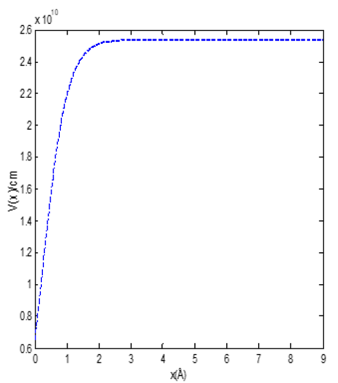
The shape of the molecular attractive potential for chlorine molecule is shown in Fig. 1. The effect of the screening parameter on the energy of the attractive potential is shown in Fig. 2. The energy varies directly with the screening parameter. However, as the screening parameter increases above 2, the energy of the system has turning point starting from the energy of the highest quantum state. In Fig. 3, we examined the effect of the dissociation energy on the energy of the molecular attractive potential. The energy of the system increases monotonically as the dissociation energy increases gradually for all the quantum states. Figures 2 and 3 are plotted using Eq. (29)

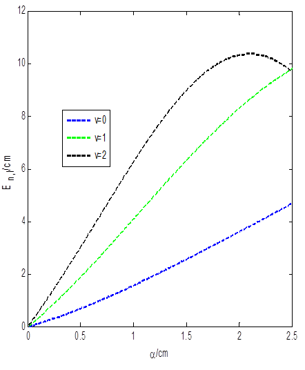
Fig. 2 Variation of energy against the screening parameter for molecular attractive potential with =μ=l=1,   λ0=2,re=0.55 and De=10.[/p]  

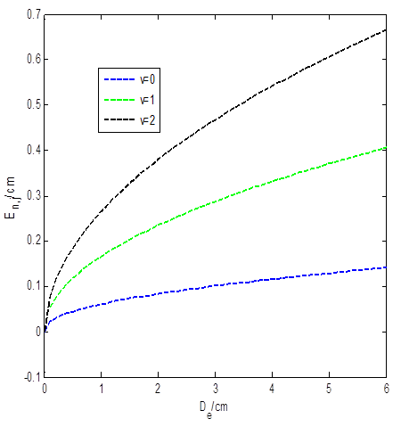
Fig. 3 Variation of energy against the screening parameter for molecular attractive potential (a) and improved Rosen-Morse potential (b) with =μ=l=1,   λ0=2, α=0.15 and re=0.55.[/p]  

The comparison of the present results and the previous results for attractive molecular potential are presented in Table 1. The present results and the previous results agreed with one another. Imputing the experimental data De=3341470cm-1, re=1.762 A,  αe=2 511cm1 , and we=255.380cm-1 into equation (29), we obtained the rotational vibrational energy for chlorine molecule. The comparison of the experimental values and the calculated values are presented in Table 2. The experimental values are obtained from ref. [19, 20]. The calculated results showed a good agreement with the observed values. To ascertain the degree of accuracy of the calculated values, we obtained the percentage deviation from the observed values. The percentage deviation for the present calculation with j = 0 is 0.0589 % while the percentage deviation with j = 1 is 0.0603 %. The percentage deviation is obtained using the formula

Table 1 Comparison of the energy of the attractive molecular potential for various quantum states and angular quantum states with =μ=l=1,   λ0=2, α=0.25 and re=0.25.[/p]  

n l De=5Present[6] De=10Present[6]
0 0 3.977598260 3.977598297 6.798286894 6.798287056
1 0
1
4.809523564 4.792524933
4.940728412 4.955213995
9.108667476 9.075571808
9.543813181 9.592230252
2 0
1
2
4.976039762 4.967085778
5.003831145 4.999752546
5.012890620 4.980612046
9.723414912 9.696564702
9.872914437 9.882375036
9.966101890 9.981247750
3 0
1
2
3
4.998604183 4.999955612
4.988391768 4.980876842
4.973213572 4.926380148
4.962051470 4.844354168
9.936060172 9.920455196
9.987095855 9.984079176
10.01504929 9.998356127
10.02737409 9.962890521
4 0
1
2
3
4
4.963711498 4.975269344
4.931818281 4.926609948
4.899233943 4.847057320
4.874254153 4.744069524
4.858672822 4.620971626
9.997844943 9.993868287
10.00275060 9.997542268
9.994948650 9.962692496
9.982639903 9.891525886
9.972505733 9.791084240

Table 2 Comparison of the observed values and calculated values of the Chlorine molecule (Cl2

v RKR (cm-1) [19] calculated results
j=0 j=1
0
1
2
3
4
5
6
7
8
9
10
279.15
833.43
1382.33
1925.79
2463.80
2996.28
3523.40
4044.80
4560.50
5070.50
5574.70
272.0144
815.8936
1359.5343
1902.9364
2446.0997
2989.0242
3531.7099
4074.1566
4616.3643
5158.3328
5700.0622
272.4928
816.3721
1360.0128
1903.4150
2446.5783
2989.5029
3532.1887
4074.6354
4616.8432
5158.8118
5700.5412

σ=100Ni=0Eca-EexEex,(43)

where, i=0Eca-EexEex, is the experimental data, Eca is the calculated value and N is the number of data points.

Conclusion

The solution of the radial Schrödinger equation was obtained under the attractive molecular potential model. It was observed that two different energy equations can be obtained under this potential. Then, one of the energy equations obtained was used to generate numerical values for chlorine molecule which perfectly agreed with the experimental values. The deviation of the calculated values from the experimental values is approximately 0.0589 % for j = 0 and 0.0603 % for j = 1 Thus, the attractive molecular potential perfectly fits the computation for Chlorine molecule.

References

1. Jia, C. -S.; Cao, S. -Y. Bull. Korean Chem. Soc. 2013, 34, 3425-3428. DOI: http://dx.doi.org/10.5012/bkcs.2013.34.11.3425 [ Links ]

2. Yanar, H.; Aydogdu, O.; Saltı M. Mol. Phys. 2016, 114, 3134-3142. DOI: http://dx.doi.org/10.1080/00268976.2016.1220645 [ Links ]

3. Bin Tang, B.; Jia, C. -S.. Eur. Phys. J. Plus. 2017, 132, 375. DOI: http://doi.org/10.1140/epjp/i2017-11657-7 [ Links ]

4. Khordad, R.; Ghanbari, A. J. Low Temp. Phys. 2020, 199, 1198. DOI: https://doi.org/10.1007/s10909-020-02368-8 [ Links ]

5. Liu, J. -Y.; Hu, X. -T.; Jia, C. -S. Can. J. Chem. 2014, 92, 40. DOI: dx.doi.org/10.1139/cjc-2013-0396 [ Links ]

6. Onate, C. A.; Akanbi, T. A.; Okon, I. B. Scientific Reports. 2021, 11, 6198. DOI: https://doi.org/10.1038/s41598-021-85761-x [ Links ]

7. Onate, C. A.; Akanbi, T. A. Result. Phys. 2021, 22, 103961. DOI: https://doi.org/10.1016/j.rinp.2021.103961 [ Links ]

8. Zhang, L. -H.; LI, X. -P.; Jia, C. -S. Int. J. Quant. Chem. 2011, 111, 1870. DOI: http://dio.org/10.1002/qua.22477 [ Links ]

9. Qiang, W.-C.; Dong, S.-H. Physics Letters A. 2007, 368, 13. DOI: doi:10.1016/j.physleta.2007.03.057 [ Links ]

10. Dong, S.-H; Qiang, W.-C. Phys. Lett. A. 2008, 372, 4789. DOI: doi.org/10.1016/j.physleta.2008.05.020 [ Links ]

11. Greene, R. L.; Aldrich, C. Phys. Rev. A. 1976, 14, 2363-2366. DOI: https://doi.org/10.1103/PhysRevA.14.2363 [ Links ]

12. Jia, C. -S.; Guo, P.; Diao, Y. -F.; Yi, L. -Z.; Xie, X. -J. Eur. Phys. J. A. 2007, 34, 41-48. DOI: http://doi.org/10.1140/epja/i2007-10486-2 [ Links ]

13. Hassanabadi, H.; Zarrinmakar, S.; Rahimov, H. Commun. Theor. Phys. 2011, 56, 423. DOI: http://www.iop.org/EJ/journal/ctpLinks ]

14. Wei, G. -F.; Dong, S. -H. Phys. Lett. B. 2010, 686, 288. DOI: http://doi.org/10.1016/physletb.2010.02.070 [ Links ]

15. Witten, E. Nucl. Phys. B. 1981, 188, 513. DOI: https://doi.org/10.1016/0550-3213(81)90006-7 [ Links ]

16. Gendenshtein, L. E. Sov. Phys. (JETP) Lett. 1983, 38, 356. [ Links ]

17. Cooper, F.; Khare, A.; Sukhatme, U. Phys. Rep. 1995, 251, 267. DOI: https://doi.org/10.1016/0370-1573(94)00080-M [ Links ]

18. Comtet, A.; Bandrank, A.; Campbell, D. E. Phys. Lett. B. 1985, 150, 159. DOI: https://doi.org/10.1016/0370-2693(85)90160-1 [ Links ]

19. Coxon, J. A. J. Quant. Spectrosc. Radial Transfer. 1971, 11, 443-462. DOI: https://doi.org/10.1016/0022-4073(71)90083-5 [ Links ]

20. Kaur, S.; Mahajan, C.G. Pramana J. Phys. 1999, 52, 459. DOI: https://doi.org/10.1007/BF02830093 [ Links ]

Received: December 26, 2021; Accepted: March 17, 2022

*Corresponding author: C.A. Onate, email: oaclems14@physicist.net

Creative Commons License This is an open-access article distributed under the terms of the Creative Commons Attribution License