Nota corta

 

Technical and economic optimum in feedlot cattle

 

Óptimo técnico y económico en bovinos productores de carne engordados en corral

 

S. Rebollar-Rebollar²*, R. R Posadas-Domínguez¹, J. Hernández-Martínez², R. Rojo-Rubio², F. J. González-Razo², E. Guzmán-Soria³

 

¹ Posgrado en Ciencias Agropecuarias y Recursos Naturales-Universidad Autónoma del Estado de México.

² *Centro Universitario UAEM Temascaltepec-Universidad Autónoma del Estado de México. Km. 67.5, carr. Toluca-Tejupilco. Col. Barrio de Santiago S/N, Temascaltepec, Estado de México. C. P. 51300. Fax. 01 716 26 652 09. *Corresponding author E-mail (samrere@hotmail.com).

³ Posgrado de Administración. Instituto Tecnológico de Celaya. Av. Tecnológico y A. García Cubas S/N. CP 38010. Celaya, Guanajuato.

 

Submitted April 07, 2010
Accepted November 05, 2010
Revised received November 11, 2010

 

Abstract

The beef cattle producers in the southern zone of the State of Mexico generally do not carry out adequate market planning of their finished steers. In addition, they lack technical and administrative management in their productive units, focused on the use of efficient input, which has prevented them from maximizing their monetary profits. The present investigation was made to estimate the technical (TOL) and economic optimum levels (EOL) of feedlot beef cattle, using two cubic production functions with decreasing marginal yields. One hundred steers of Bos Taurus x Bos indicus were used, with Live Weight at the start of fattening of 290 ± 15 kg, age 21 to 24 months, fattened in feedlots during 93 days consuming a totally mixed diet (Crude protein: 133.33, FDN: 237.44, FDA 114.33 g/kg DM and 2.62 Mcal/kg of DM of metabolizable energy) To estimate both functions (TOL and EOL), weight gain was considered as independent variable. For the first production function, feed intake was taken as independent variable and in the second function, time defined in days. For the first production function the TOL was 475.04 and the EOL was 473.94 kg Live Weight; with a daily feed intake of 12.58 and 12.36 kg/day. For the second production function the TOL was 475.01 and the EOL was 460.21kg of Live Weight, with a period of 93.29 and 77.21 days. The optimal point of sale and the maximum gain is obtained with the second production function, when the animals reach a Live Weight of 460.21 kg during a feeding period of 77.21 days.

Key words: beef cattle; production functions, technical optimum, economic optimum.

 

Resumen

Los engordadores en corral de bovinos productores de carne en la zona sur del Estado de México, generalmente no realizan una planeación adecuada de venta al mercado de sus novillos finalizados. Asimismo, carecen de un manejo técnico y administrativo en sus unidades productivas, enfocado con el uso eficiente de insumos, lo que ha impedido que maximicen sus ganancias monetarias. La presente investigación se realizó para estimar los niveles óptimo técnico (NOT) y económico (NOE) de bovinos engordados en corral, utilizando dos funciones de producción cúbicas con rendimientos marginales decrecientes. Se utilizaron 100 novillos Bos taurus x Bos indicus, Peso Vivo a inicio de la engorda de 290 ± 15 kg, edad 21 a 24 meses, engordados en corral durante 93 días consumiendo una dieta totalmente mezclada (Proteína cruda: 133.33, FDN: 237.44, FDA 114.33 g/ kg MS y 2.62 Mcal/kg de MS de energía metabolizable). Para estimar ambas funciones (NOT y NOE), la ganancia de peso fue considerada como variable dependiente. Para la primera función de producción el consumo de alimento fue tomado como variable independiente y en la segunda el tiempo definido en días. Para la primer función de producción el NOT fue de 475.04 y el NOE de 473.94 kg de Peso Vivo; con un consumo de alimento de 12.58 y 12.36 kg/día. Para la segunda función de producción el NOT fue 475.01 y el NOE de 460.21 kg de Peso Vivo, con un periodo de 93.29 y 77.21 días. El punto óptimo de venta y la máxima ganancia se obtiene con la segunda función de producción, cuando los animales alcanzan un Peso Vivo de 460.21 kg durante un periodo de alimentación de 77.21 días.

Palabras clave: bovinos carne; funciones de producción; óptimo técnico; óptimo económico.

 

INTRODUCTION

Beef production is the most widely practiced productive activity in the rural sphere. It uses slightly over 110 million ha, which represents 60.00 % of the national surface; the production systems range from the most highly technical and integrated to the traditional systems. Beef production has been maintained as the axis for different production tendencies and the meat market in Mexico (Ruiz et al., 2004).

In Mexico cattle is developed under diverse agro-ecological conditions, mainly influenced by climatic and technological factors, management systems and by exploitation purpose. This micro-climatic variability does not permit homogeneity in production. Similarly, the applied technology is variable, including traditional production systems and those that use state-of-the-art technology (SAGARPA, 2010). In general terms, the conditions under which Mexican cattle production are carried out are extensive, although finishing in feedlots is also practiced. This type of production is limited, due to the fact that it implies higher feeding costs than extensive production (Herrera et al., 1998; Ruiz et al., 2004).

However, in the last decade, the feedlot production system has made great progress, especially in the national supply of finished cattle, rising from 20.00 % in 2004 to 35.00 % in 2008. Furthermore, the multiplication of this productive system, mainly in the temperate region and the north-central zone of the country, has brought considerable advances in growth and production to this system. This strengthening and advance is due to the advantages of finishing cattle under the feedlot system, given that its operation requires a minimum use of land extensions, which is added to good acceptation and commercialization in the markets of national consumption. These advantages, along with the change in demand of consumers of meat from pasture fed animals to meat with white fat from feedlots, has meant the growth reflected in the last decade of the feedlot production system (FIRA, 2008).

In 2008, according to information of SAGARPA, Mexican beef carcass production supplied nearly 39.00 % of the total value of meats, followed by poultry (35.50 %) and in third place, pork with approximately 23.00 %. The production of sheep, goat and turkey lag behind, which together supply approximately 3.00 % of meat production. The highest volumes of beef meat production are obtained during the months of October to December, the highest point being in November, which is invariable due to the abundant production of fodders, consequence of the rainy season and to a higher consumption in this period, which has to do with natural consumption conditions. In the same year, the principal producers of beef meat in Mexico were Veracruz (14.60 %), Jalisco (10.80 %), Chiapas (6.10 %), Chihuahua (5.10 %), Sinaloa (4.70 %), Baja California (4.70 %) and Sonora (4.50 %), which together supplied 50.50 % of the national total (SIAP, 2010).

In the same year, the State of Mexico registered 559.00 thousand meat steers and supplied 78 795 t of meat (2.50 %) to the national production. In districts, Atlacomulco occupied first place with 21.66 % of the state production, followed by Tejupilco (17.46 %), Texcoco (12.63 %), Toluca (12.59 %), Coatepec Harinas (10.84 %), Zumpango (9.70 %), Jilotepec (8.08 %) and Valle del Bravo (7.00 %) (SAGARPA-SIAP, 2009). In these districts there are two major production systems: 1) cow-calf or semi-extensive, with fattening in native pastures complemented with balanced diets; 2) feedlot cattle production, fed with mixed diets and commercial feed during 90 to 105 days. There are native cattle crossed with Cebú, Brown Swiss, Charolais, Angus and Beefmaster of the U.S. (SAGARPA, 2004).

The seedstock systems are concentrated in the region of Tejupilco, one of the warmest zones of the state, where the lack of forage during the dry season is a limiting factor, which justifies the feedlot system, although recent establishments of pastures with Prairie grass (Andropogon gayanus), African Star Grass (Cynodon plectustachus) and Chontalpo (Brachiaria decumbes) have reduced this limitation, there are forage conservation techniques and supplements to improve the feeding of cattle (SEDAGRO, 2007).

The use of production functions in the national livestock sector has been of great importance for the optimum assignation of resources in the productive processes: Their estimation makes it possible to derive technical-economic recommendations that can be applied by producers for a better use of the productive inputs (Espinosa, 2001).

The inadequate use of inputs on the part of the producers does not necessarily coincide with technical or economic recommendations that would allow them to maximize their profits. Therefore, the objective of this investigation consisted of determining the technical-economic efficiency of productive resources focused on inputs that are utilized, principally feed and obtained product (finished cattle).

 

MATERIALS AND METHODS

The study was carried out in the locality of Almoloya de Granadas, Tejupilco, State of Mexico, located to the southwest of the entity, at 18° 54' 30" N and 100° 09'00" W; altitude 1 540 masl, minimum and maximum annual temperature of 15 and 30°C, respectively; precipitation 1 014 mm annually; semi-warm climate with rains in summer (INEGI, 2003). The information came from a production unit dedicated to intensive fattening of cattle in feedlots. The data of feed intake (quantified daily from the feed offered minus rejected feed), weight gain (quantified with the aid of a portable electronic scale, Gallagher model SmartScale 200, 2 t capacity) and days of fattening, were taken from 100 steers which were managed homogeneously, and given that no effect (treatment) was measured as a conventional experimental design, the sample was considered unique. In this sense all of the animals consumed a totally balanced mixed diet according to the tables of the NRC (2000) (Table 1) that satisfied the nutritional requirements of the animals during the finishing period; the estimated cost of the diet was 2.74 $/kg of dry matter.

 

The data obtained during the study period, such as input cost (feed) and the sale prices of the animals were used to feed the econometric models that are specified below:

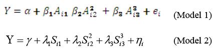
Where:

Y = Live weight of the animals, in kilograms

Α = Intercept of the function

β_i =Parameters to estimate; i = 1, 2, 3

Aⁿ_ij = Term of stochastic, random or statistical error; with normal standard distribution, variance σ² and σ_ij = 0, for every i≠j

λ = Parameters to estimate; i = 1, 2, 3

γ = intercept of the function

Sⁿ_ij = Independent explicative or predetermined term of the function; i and j = 1, 2, 3; n = 1, 2, 3, and indicates the number of weeks of fattening.

(1) and (2) should comply with the characteristics of any production function, principally of the concavity of the curve, with which it is possible to mathematically derive the technical and economic optimums.

The technical optimum for (1) is: MP = 0, that is;

The economic optimum for (2) is: , or MP = Px/Py; Px and Py are the prices of the input (feed) and of the product (live weight of the animals). It is expected that at least one of the non-linear terms of the function will be less than zero.

Similarly, the technical optimum or maximum production in (2) is:

The economic optimum for (2) is:

In this case, S suffered a conversion to kg of feed to determine the technical and economic optimum in days of fattening.

The models were estimated by means of the procedure of general linear models (GLM) of SAS (2001).

 

RESULTS AND DISCUSSION

The productive response of the animals, in terms of weight gain, is specified in Table 2. At the start of the fattening process a first stage was observed, which was found in weeks one to four, and was characterized by small increases in weekly weight gains, which is explained by the adaptation of the cattle to the diet. However, it is observed that from the fifth to the ninth week the weight gain of the cattle followed an increasing tendency, and it was in this stage where the period of highest efficiency appeared in the transformation of the variable input to product (weight of the cattle). After week 11, decreasing but positive weight gains occurred; that is, as fattening time transpired, the variable input (feed) was increasingly less efficient in transformation to product, to the point where each additional unit of variable input (feed) presented lower values to the unit; this is due to the fact that cattle production, as with other productive processes, is subject to the Law of Diminishing Returns.

 

The information of Table 2 was used to feed the econometric models and to estimate the production functions, both for the feed variable (F) and for the time variable expressed in days (S), which made it possible to obtain the equations and estimators for each parameter used in both models, as well as the behavior of the data as a function of the time transpired and feed consumed by the animals. From this information, it was possible to mathematically derive the level that guarantees the maximum production (TOL) and the maximum economic gain (EOL). The equations for each model were as follows and were obtained from the output of SAS:

The F calculated (Fc) in model (1) and model (2) was 157.42 and 8 401.63 and implies, for each one of the models, the number of times that the Mean Square of the Regression (MSR) contains the Mean Square of the Error (MSE). On the other hand, the values in parenthesis of both models are the standard errors of the estimators; which when multiplied by two give a result which is less than the value of the estimator, which guarantees the statistical significance (Gujarati, 2004); whereas the results of the second row for such models, refer to the statistic t (Student) calculated (tc) for each estimator. The R² (coefficient of determination or adjustment) in both models was 0.979 and 0.999, that is, that 97.9 ad 99.9 % of the total variable in the weight of the cattle was explained through the regression models and represented a satisfactory level of explanation of the model as a whole. The signs that precede the coefficients of the estimated model, were those expected (Doll and Orazem, 1984), thus the model is significant from the statistical and economic viewpoint; result that permitted the estimation of the technical optimum level (TOL) economic optimum level (EOL).

 

Economic analysis

The sign (negative) that precedes the variables F and W for each model indicated the presence of two cubic production functions with decreasing marginal yields; therefore, the additional application of one more unit of variable input (feed) and the time that transpires in fattening, will lead to progressively lower increments in the weight of the animals. In this sense and under the given conditions, the value of the ordinate at the origin (289.94) cited in model (1), did not have economic significance, and was far from the group of data observed, thus it cannot be interpreted as the weight of the animals at the start of fattening, when the independent variable (F) has a value of zero. On the other hand, the value of the intercept (291.48) cited in model (2) indicated the initial weight of the cattle when (W) takes a value equal to zero, which coincided with the average weight (290 kg) of the animals at the start of fattening.

 

Technical optimum or maximum production level (TOL)

The technical optimum is that in which the production function finds its maximum, in terms of physical production volume (Lanfranco and Helguera, 2006). This is always found above the economic optimum, and represents a production level where input prices do not intervene. Once the production functions have been determined, it is possible to indicate that the production at the beginning will increase to a higher velocity of transformation of the variable input in total product to the degree in which an additional unit of the same input (feed) is increased; but it will reach a point where the weight of the cattle will present a decreasing marginal yield, and it is in this level where the maximum weight or technical optimum will be obtained. Mathematically, the value of the variable input that maximizes production is found through the first derived from the function equaled to zero.

Thus, by substituting the estimated values of each equation in models 1 and 2, and subtracting the total cost of the variable input (feed) in the entire fattening process, the Live Weight (LW) of the animals was obtained, where maximum production is reached (TOL) along with maximum economic gain (EOL). According to the procedure described (Rebollar et al., 2008a), in model (1) (where Y or Live Weight of the animals was a function of the feed (F) that the animals consumed throughout the fattening process), when the equation in (1) was derived mathematically, it was estimated that F took a value equal to 88.10 kg of feed per week; that is, 12.58 kg of daily intake; that is, 1 174.12 kg of feed in the entire fattening period, which guarantees the TOL. For model (2) (where Y was a function of the time expressed in days), S took on a value equal to 93.32 d, with a feed intake of 86.53 kg per week; that is, 12.36 kg of daily intake; that is, 954.42 kg of feed in the entire fattening period, which guarantees the EOL. With the above, the first model indicated that the cattle could reach their maximum weight (TOL, 475.04 kg) and their maximum gain (EOL, 473.94 kg) when they consume 88.10 and 86.53 kg per week, respectively. For the second model (93.32 days), the TOL and EOL was achieved when the animal reached a Live Weight of 475.01 kg, and in a fattening period of 93.29 and 77.21 days (Table 3).

 

The results of Table 4 make it possible to observe the behavior in the variables of the production function. The total product (TP), understood as the weight of the cattle obtained for different levels of feed intake, begins, grows and reaches its maximum value when A (variable input) is equivalent to 88.10 kg, which represented the TOL; from this value, the TP is increasingly lower. On the other hand, when A is equal to 82 kg, the mean product (AP), which represents the production level obtained by the producer per unit of variable input used, it is maximum and then descends. Similarly, the marginal product (MP), defined as the change in the TP (in absolute value) related to the increase of one unit of variable input (feed), was maximum when A had a value of 58 kg, after this level the growth rate of the MP was lower. The identification of the production stages is given by the elasticity (Ep), which is defined as the percentage change experienced by production as a result of a percentage change in the level of utilization of a variable input; which also can be expressed as the quotient between the marginal product and the mean product (Ep=MP/AP). Thus, by definition, stage I begins from zero to where the Ep is equal to 1.12 (maximum mean product), stage II (profitable stage of the productive process) begins from the point where the AP is maximum to the point where the Ep takes a value of 0.10, after this level, it corresponds to stage III of production; that is, where the MP is decreasing and to negative rates. In the above mentioned Table, the value of the technical optimum was subject to a test with an input unit prior to and after 88.10 kg, mathematically proving that the obtainment of the TOL is only guaranteed at this level.

 

Figure 1 shows the graphic representation of the production function and its response to feed, as well as the production stages. In stage I, weight gain was higher with respect to stages II and III; in this stage, the yields are increasing to rates higher than the unit, thus the producer should not sell his cattle at this stage, given that it is when the variable input (feed) presents its highest efficiency in transformation to product. Additionally, this stage ends at where the AP is maximum. In the second production stage (fattening), the cattle continue to gain weight, but at positive decreasing rates and the stage ends at the point where the derivate of the production function is equal to zero (MP = 0). Under the focus of economic theory, at some point of this part of the curve the optimum of sale (level of maximum monetary gain) is located, which in this investigation was 86.53 kg of feed and a Live Weight of the animals of 473.94 kg. At stage III, although they continue to consume feed, their weight gains are lower (to negative decreasing rates); therefore the producer should not continue to maintain his animals in confinement, given that the cost of producing one kilogram more of weight would be higher than what he receives for its sale. In other words, the MC > MI, being in this stage when the gains of the producer would decrease the longer his animals are kept in the corral. By definition, in stage I the MP is higher than the AP and they are equaled at the point where the AP is maximum, afterwards, the MP continues to decrease until reaching negative values (after the start of stage III of production).

 

Economic optimum level (EOL) or of maximum gain

The economic optimum refers to the production level in which the benefits are maximized (total income), and depends on the price of the products generated by the producers and of their cost structure (Lanfranco and Helguera, 2006), thus it should be produced where the MP of the variable input is equal to its marginal cost (MC), defined as the increase in the total cost necessary for producing an additional unit of the product. Given that the yields are decreasing, or, when the value of the derivate at this point is equal the ratio of prices of the input and the product.

To estimate the values in the independent variables A and S, within models 1 and 2, the respective derivates were used, which permitted the estimation of both the TOL and the EOL, as well as the net gains for each level, considering only the input variable (feed). Thus, the EOL for model 1 was obtained when the MP = Px/Py: that is, when the first derivate of the function (the MP) was equal to the relationship of prices of input and the product. For Py (sale price of live cattle), a price of $20.00 per kg was used, and like Px, the price per kilogram of variable input (feed) administered to each animal, of $ 2.74. With this price information, the total income for each model was estimated. Thus, the net gain at the EOL, in both models, was higher with respect to when the animals were taken to the maximum weight or TOL. With these results, it is confirmed that the maximum production or TOL does not necessarily imply the obtainment of the maximum economic gain, given that a better combination is given at the EOL, in the cost of the variable input (feed), with the obtained product; thus obtaining a higher income for the producer, than what would be obtained when the animals are commercialized at the TOL. It should be mentioned that the optimum sale weight of the animals, which guarantees the maximum economic gain, could vary due to price fluctuations that could occur in the markets of inputs and of the product.

The result of the last column of Table 5 was obtained by the arithmetic difference in the gains at the level of each variable. For example, in variable A (feed) and S (weeks of fattening), if the producer should opt to take the animals to the maximum LW or TOL, then at the moment of sale, he would cease to gain 225.68 and 381.66 pesos per animal.

 

CONCLUSIONS

The second production function used to estimate both the TOL and the EOL gave the best gain and economic profit; given that it is where the best combination of prices is obtained, both of input and of product. In practical terms, the beef cattle producer should send his animals to market with a live weight of 460 kg or at 77 days of fattening. It is important to take into account that the economic optimum level is sensitive to the fluctuations in the price changes, both of input and of products, thus the weight at market could vary.

 

REFERENCIAS

Cochran, W. G. 1984. Técnicas de Muestreo. Ed. C. E. S. A. México, D. F. 513 p.         [ Links ]

Doll, J., and F. Orazem. 1984. Production Economics. Theory with Applications. Second Edition. John Wiley Sons, Canadá. 457 p.         [ Links ]

Espinosa, G. J. A. 2001. Productividad del sistema-producto pecuario en México. Técnica Pecuaria Méx. Vol. 39 (2): 127-138.         [ Links ]

FIRA (Fideicomisos Instituidos en Relación con la Agricultura). 2008. Información del sector. http://ganaderia.fira.gob.mx. (Consulta el 07 de abril de 2010).         [ Links ]

Gujarati, D. N. 2004. Econometría. Cuarta Edición. Editorial Mc Graw Hill. México, D. F. 972 p.         [ Links ]

Herrera, H. J. G., Mendoza, M. G., Hernández, G. A. 1998. La ganadería familiar en México, Instituto Nacional de Estadística Geografía e Informática (INEGI). Aguascalientes, Ags. 80 p.         [ Links ]

INEGI (Instituto Nacional de Estadística, Geografía e Informática). 2003. Anuario Estadístico del Estado de México. Aguascalientes, Ags. México. 731 p.         [ Links ]

Lanfranco, C. B., y L. Helguera, P. 2006. Óptimo técnico y económico. Diversificación, costos ocultos y los estímulos para mejorar los procreos en la ganadería nacional. Revista INIA 8: 2-5.         [ Links ]

National Research Council. 2000. Nutrient Requirements of Beef Cattle. Academic Press. USA. 248 p.         [ Links ]

Rebollar R. S., J. Hernández, M., R. Rojo, R., F. J. González, R., P. Mejía, H., D. Cardoso, J. 2008a. Óptimos económicos en corderos Pelibuey engordados en corral. Universidad y Ciencia 24 (1): 67-73.         [ Links ]

Rebollar R. S., G. Gómez, T., J. Hernández, M., R. Rojo, R., F. J. González, R., F. Avilés, N. 2008b. Determinación del óptimo técnico y económico en una granja porcina en Temascaltepec, Estado de México. Ciencia Ergo Sum 14-3: 255-262.         [ Links ]

Ruiz F. A., M. L. Sagarnaga, V., J. M. Salas, G., V. Mariscal, A., H. Estrella, Q., A. Ruiz, F., M. González, A., y A. Juárez, Z. 2004. Impacto del TLCAN en la cadena de valor de bovinos para carne. Universidad Autónoma Chapingo. Enero 2004. http://www.cnog.com.mx/.../Impacto%20del%20TLCAN%20en%20la%20cadena%20Bovinos. (Consulta el 24 de junio de 2009).         [ Links ]

SAGARPA (Secretaría de Agricultura, Ganadería, Desarrollo Rural, Pesca y Alimentación). 2004. Situación Actual y Perspectiva de la Producción de Carne de Bovino en México. Coordinación General de Ganadería. México, D.F. 34 p. http://www.sagarpa.gob.mx/ganaderia/publicaciones. (Consulta el 24 de agosto de 2009).         [ Links ]

SAGARPA-SIAP (Secretaría de Agricultura, Ganadería, Desarrollo Rural, Pesca y Alimentación-Servicio de Información Agroalimentaria y Pesquera). 2009. Información Estadística: Distrito de Desarrollo Rural 076) de Tejupilco, Estado de México. http://www.sagarpa.gob.mx/Dgg. (Consulta el 18 de septiembre de 2009.         [ Links ]

SAGARPA-SIAP (Secretaría de Agricultura, Ganadería, Desarrollo Rural, Pesca y Alimentación-Servicio de Información Agroalimentaria y Pesquera). 2010. Estudios de Situación actual. http://www.sagarpa.gob.mx/Dgg. (Consulta el 06 de octubre de 2010).         [ Links ]

SIAP (Servicio de Información Agroalimentaria y Pesquera). 2009b. Información estadística sobre ganadería. http://www.siap.gob.mx. (Consulta el 19 de noviembre de 2009).         [ Links ]

SIAP (Servicio de Información Agroalimentaria y Pesquera). 2010. Información estadística sobre ganadería. http://www.siap.gob.mx. (Consulta el 06 de octubre de 2010).         [ Links ]

Samuelson, P. A., y D. Nordhaus, W. 2002. Economía. Decimoséptima Edición. Ed. Mc Graw Hill. Madrid, España. 701 p.         [ Links ]

SEDAGRO (Secretaría de Desarrollo Agropecuario). 2007. Programa Institucional. Gobierno del Estado de México. http://www.sedagro.gob.mx . (Consulta el 12 de octubre de 2009).         [ Links ]

SAS. 2001. The SAS System for Windows. Release 8.2.SAS Institute Incorporation, Cary, NC, USA. 558 p.         [ Links ]