


 nueva página del texto (beta)
 Inglés (pdf)
 Artículo en XML
 Referencias del artículo
 Enviar artículo por email
 Citado por SciELO
  Similares en
SciELO
Similares en
SciELO 
 Permalink
1. Introduction
Optical techniques have been shown along the years to be very effective for vibration measurement (Ostrovsky et al., 1991; Cloud, 1998). Excepting few cases exploring geometrical properties of diverging optical beams (Remo, 1996), the great majority of the optical measurement techniques use interferometry. Doppler Laser Vibrometry (DLV) is a very well-established interferometric method suitable for a myriad of applications (Freschi et al., 2003; Frejlich et al., 2000). In DLV the vibration mapping is obtained upon continuously tilting a mirror in order to scan the vibrating surface. Time average holography and time average digital speckle pattern interferometry (DSPI) allow whole-field analyses and are very suitable for micro-vibration measurements. The dynamic range of those techniques can be enlarged with the help of stroboscopy (Hariharan et al., 1987; Watrasiewicz & Spicer, 1968; Yang et al., 2009; Yang et al., 2014) and phase-modulated reference beams (Barbosa & Lokberg & Høgmoen, 1976; Muramatsu, 1997). If the vibration amplitudes are too large to be measured by standard time average methods, double-pulse (Pedrini et al., 2002) or high-speed camera holography (Fu et al., 2007; Pedrini et al., 2006) are also useful tools for this purpose, even enabling the analysis of non-harmonic vibration phenomena. In the conventional time-averaged holographic and speckle methods the fringe pattern can only be observed and evaluated if the regions of the surface vibrate with different amplitudes and preferably when there is a nodal region. Hence, those techniques have low sensitivity or are even ineffective if all the points vibrate with the same amplitude, or if the amplitude values are so close to each other that no distinguishable fringes can be visualized.
The oblique incidence and projection of structured light is widely used for 3D reconstruction of surfaces. This technique is employed in fields like facial recognition (Guo & Liu, 2007), dentistry (Ireland et al., 2008; Múnera et al., 2012), reverse engineering (Chao-hui et al., 2005) and microscopy (Yin et al., 2015), among many others.
In the basic configuration of fringe projection metrology it is not possible to study dynamic phenomena without high-speed cameras because of the obvious lack of fringe visibility due to the object movement. Hence, in order to analyze dynamic processes by fringe projection with standard cameras there must be a way to freeze the fringe pattern. The images of projected fringe patterns acquired by high-speed cameras have also been used for temporal vibration analyses: in (Fu, 2010), the vibration of low-frequency vibrating object was studied by projecting a sequence of fringe patterns produced by a moving grating and captured by a high-speed camera; Talbot fringes generated by a Ronchi grating were projected and analyzed by Fourier Transform to obtain the whole-field time-resolved vibration map on an Aluminum cantilever (Rodriguez-Vera et al., 2009). Temporal Fourier transform profilometry (TFTP) (Zhang et al., 2019; Zhang et al., 2020) combined with a mechanical light chopper was used for dynamic profilometry.
In this framework the present article proposes an alternative and simple approach to use interferogram projection in order to freeze and measure out-of-plane vibration amplitudes of flat or nearly flat surfaces in the millimeter and submillimeter range. The interference fringes are generated by a Twyman-Green interferometer (TG). In the first experimental configuration one of the TG mirrors is supported by a piezo-electrical transducer in order to phase modulate one of the interfering beams, resulting in a jiggling interference pattern when the illuminated surface does not vibrate. Hence, the interferogram oscillation due to the surface vibration can be compensated by the oscillation caused by the phase modulation of the TG. We derived a mathematical expression which provides the vibration amplitude of the studied surface as a function of the vibration amplitude of one of the mirrors in the TG.
In a second experiment the illuminating fringe pattern is amplitude-modulated in time with the use of a vibrating Fabry-Perot etalon (FBE). The resulting stroboscopic illumination manages to register the fringe pattern at a fixed position. The vibration amplitude is then retrieved by scanning the phase of the FBE, or by chopping the illuminating beam with a slightly different frequency than that of the vibrating object. In the experiments we analyze the vibration of a circular rubber membrane and a circular plastic plate. The vibration of a flat rectangular plastic plate and of a formica bar was also studied. All the objects were excited by a loudspeaker. In both configurations, static fringes were easily achieved with effective, simple and low-cost experimental solutions, so that drawbacks of using mechanical choppers (with a large inertia and a limited frequency range) and expensive high-speed cameras are overcome.
This article is organized as follows: in section 2 we describe the measurement principle of the methods and derive the expressions to obtain the vibration amplitude. In section 3 the experiments are described and the results are discussed. The concluding remarks are presented in section 4.
2. Vibration analysis by fringe projection
Consider the oblique incidence of a fringe pattern onto a planar surface. The fringes are originated from a Twyman-Green interferometer whose mirrors are slightly misaligned such that the distance between two adjacent and parallel fringes is d. If the angle of incidence is θ, the projected fringe pattern viewed from a direction perpendicular to the surface has a spatial period of d/cosθ.
Hence, the fringe pattern can be written as
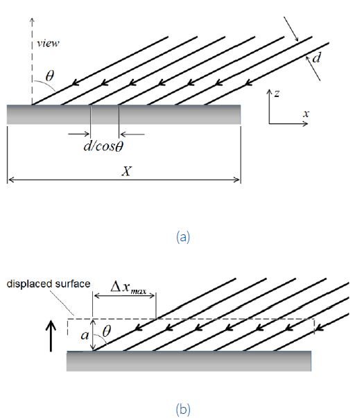
Figure 1 Fringe projection onto the surface a - in the equilibrium position and b - after a displacement a.
If the surface vibrates along the z-direction, perpendicular to the surface, the fringes will appear to the observer as oscillating along the x-axis. From Figure 1b one concludes that a surface displacement α along the z-axis corresponds to a maximum lateral fringe displacement of
where is the phase of the vibrating object.
2.1. Phase-modulated fringe pattern
Consider now that one of the TG mirrors is supported by a piezoelectric transducer (PZT-M) which makes the mirror vibrate according to
Hence, due to the simultaneous surface vibration and the TG phase modulation the total fringe displacement is
Depending on the values of a, APZT , ω, Ω and the phases, the resulting fringe pattern may appear as blurred or indistinguishable fringes; the fringe pattern can get static again
and
Hence, the from equations (1-3) the vibration amplitude of the surface is written as
Equations (3a) and (3c) determine the conditions for fringe stabilization. By achieving these conditions, both the phase and the vibration amplitude may be determined from equations (3a) and (4), respectively. This procedure will be explained in detail in section 3.1.
2. 2. Stroboscopic illumination
Suppose that the laser beam with intensity I0 impinging the TG is amplitude-modulated. This can be accomplished e.g. if the beam propagates through a Fabry-Perot etalon (FBE) in which one of the mirrors vibrates according to according
Where
where
The measurement principle is based on an heterodyne approach. When the laser is modulated with a frequency
Equation (6) shows that the interferogram appears to oscillate with a beat frequency
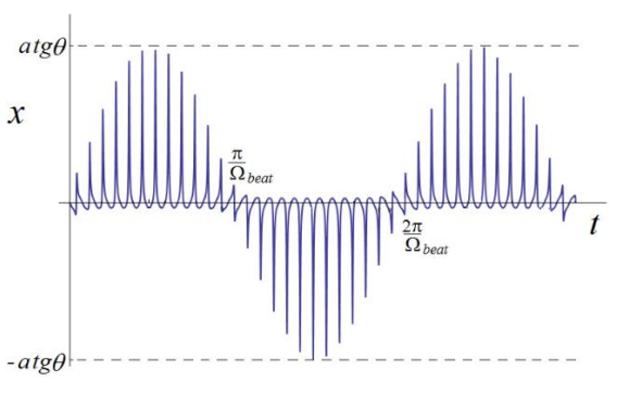
Figure 2 Position of a surface vibrating at frequency ω illuminated by a fringe pattern pulsed with frequency
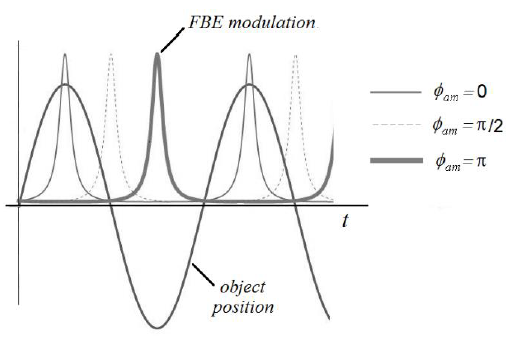
An alternative way for measurement works with the FBE modulator chopping the light at the same frequency as the object vibrates, as illustrated in Figure 3: the sinusoidal curve represents the position of a given point P on the vibrating surface as a function of time, while the spiky curves show the modulated light intensity at the FBE output, for
3. Experimental setup and results
3.1. Phase-modulated interferogram
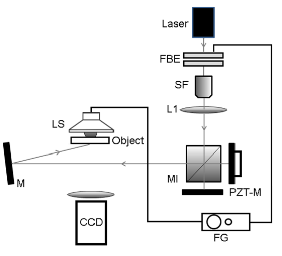
Figure. 4 shows the beam of a 532-nm frequency-doubled diode pumped solid state laser filtered by a spatial filter SF and focused by a positive lens L1 on both mirrors of the TG. The beam illuminates the TG to get the interference fringes which illuminate the object after being reflected by mirror M. The incidence angle onto the vibrating surface is
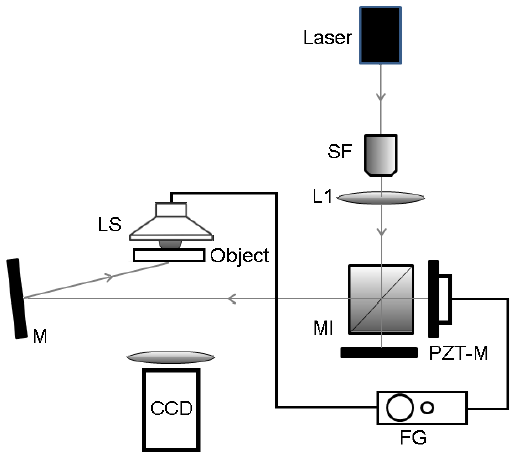
Figure 4 Optical setup: SF, spatial filter, L1, lens; TG, Twyman-Green interferometer; PZT-M, piezoelectrically moved mirror; FG, function generator; LS, loudspeaker; M, mirror; CCD, camera.
When the object vibrates and the PZT-M is off the fringes covering the object surface appear blurred and even completely indistinguishable. By exciting the PZT-M with the same frequency as the object, the fringe visibility starts enhancing as the driving PZT signal is properly adjusted and gets closer to the ideal value. However, adjusting the PZT-M amplitude only is not enough to stabilize the fringes. As it can be seen from equation (3), the phase ϕpzt must be chosen by properly setting the function generator.
Plastic membrane - Figure 5a shows the plastic membrane partially illuminated by the interferogram when both the PZT-M and the loudspeaker are off V
LS
= 0, so that the fringes can be seen with maximum visibility. In this case, the average spatial period is d = 4.2 mm. The form of the fringes is mainly due to the membrane shape and/or to the spherical wavefronts in the Twyman-Green interferometer and is irrelevant in the analysis. The LS is then excited by a 320-Hz sinusoidal signal with amplitude V
LS
= 1.000 V, which causes the fringes to get totally blurred, as shown in Figure 5b. At this frequency the PZT-M response is R
PZT
= 298.8 nm/V. Figure 5c shows also a blurred interferogram resulting from the membrane vibration when the PZT-M is driven by a 320-Hz sinusoidal signal with amplitude V
PZT
= 0.270 V, which corresponds to a vibration amplitude of
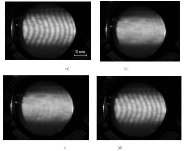
Figure 5 Study of the plastic membrane vibrating at 320 Hz for a - unperturbed membrane; b - vibrating membrane and PZT off; c - vibrating membrane and PZT on for
Plastic plate - this plate was attached to the LS core by an adhesive tape. By exciting the LS with a VLS = 1.200 V signal (PZT-M off) at 56.0 Hz, the low visibility fringe pattern can be seen in Figure 6a. For VLS = 0.150 V and
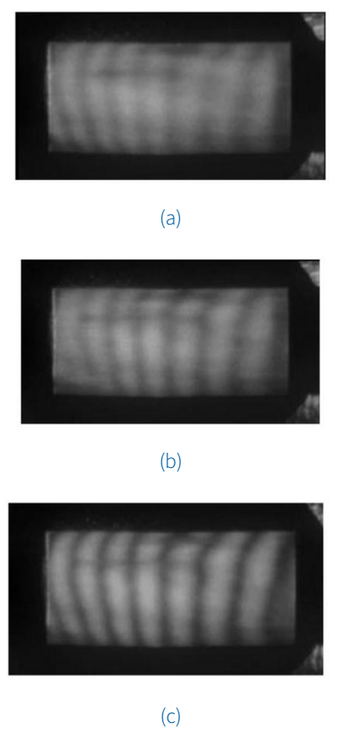
Figure 6 Study of the plastic plate vibrating at 56.0 Hz for a - vibrating plate and PZT off; b - vibrating membrane and PZT on for
Our method does enable also to measure the vibration of surfaces that do not have the same amplitude and/or phase. In the following we show qualitative experiments to demonstrate that inhomogeneous visibility changes enable identifying and measuring local vibration amplitudes. Figure 7a shows a rubber membrane with both the LS and the PZT-M peripheral part of the membrane the fringes remain with high visibility. The intensity level shown by the arrow at the right side of the figure confirms the low visibility of the fringes. By adjusting the PZT-M driving voltage amplitude to 1.210 V and its phase to 0.10 rad one obtains an interferogram whose visibility at the membrane center is highest as shown in the interferogram and the intensity level of Figure 7c. In this case, due exclusively to the PZT-M vibration the fringe visibility becomes low at the membrane periphery. Hence, once the PZT-M response at 63 Hz is known, its vibration amplitude is obtained and the local vibration amplitude is determined with the help of equation (4).
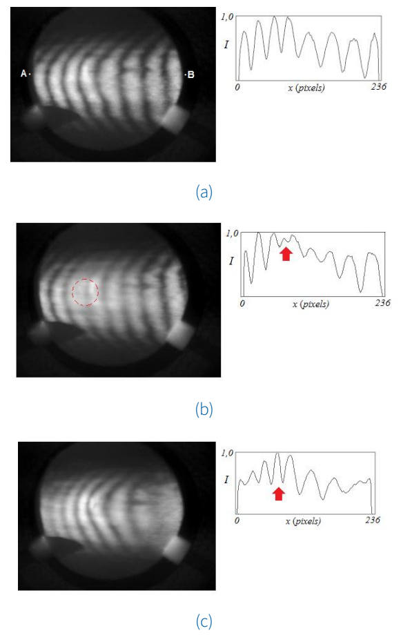
Figure 7 Vibration of the rubber membrane at 63 Hz for a - unperturbed membrane; b - vibrating membrane and PZT off; c - vibrating membrane and PZT on for
For the sake of comparison, in Figure 7a at the vicinity of the red arrow the fringe visibility defined in section 2.1 was estimated to be m = 0.38, while in Figure 7c the visibility was estimated as m = 0.32 in the same region. This discrepancy can be mainly attributed to the fact that the object is likely to vibrate at more than one frequency.
A similar testing carried out with a formica bar is shown in Figure 8. Figure 8a shows the unexcited bar, and Figure 8b shows the bar excited by a 60-Hz, V LS = 2.700 V, signal with V PZT = 0. The blurred fringes surrounded by the high visibility ones evidence that the central-right side of the bar vibrates with maximum amplitude, while the lateral parts remain still.
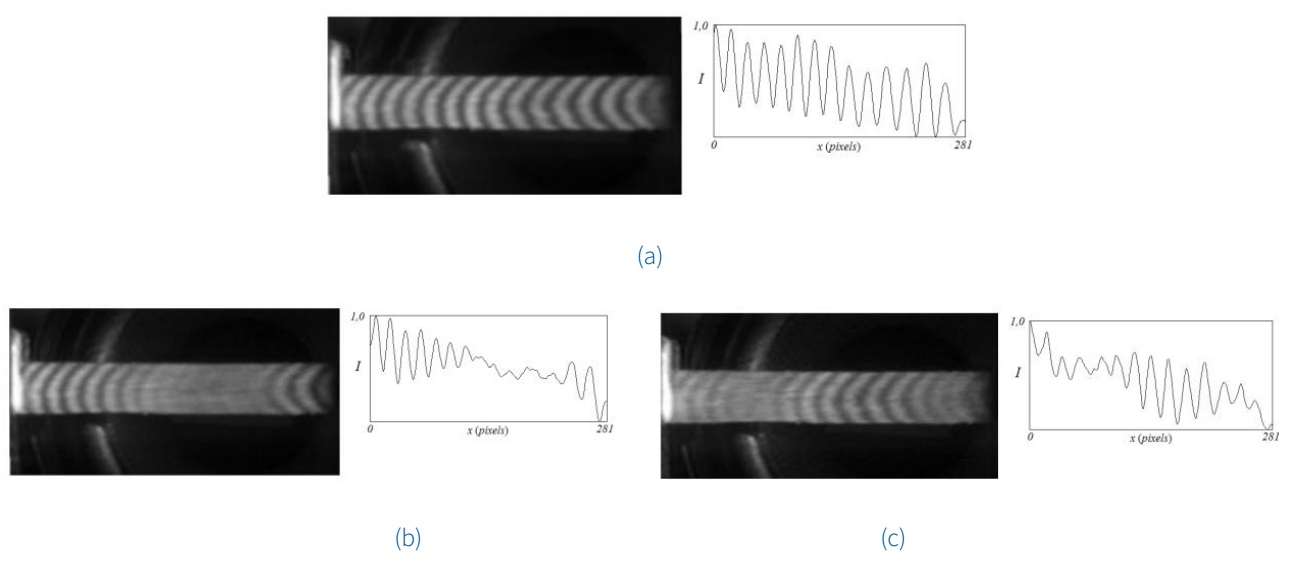
Figure 8 Vibration of the formica bar at 60 Hz for a - unperturbed bar; b - vibrating bar and PZT off; c - vibrating bar and PZT on for
As the TG is phase modulated such as V
PZT
= 1.400 V and
Some parts of the object may eventually vibrate with different phases - which was not observed in our experiments. In this case, the conditions imposed by equations (3a-c) cannot be fulfilled for the whole vibrating surface. If two adjacent parts of the object vibrate with different phases, and if the system is adjusted to get the interferogram of one of them is stable, the other part will appear blurred. The fringes of this part will only have a high visibility upon a new phase adjustment. Hence, the relative phases of these two parts will be obtained through equation (3a).
From equation (4) it is possible to estimate the sensitivity of the method. The interferogram spatial period d at the TG output is
3.2. Stroboscopic illumination
In this case the optical setup is basically the same as the one of Figure 4, except by the insertion of a home-made FBE in the beam path, as shown in Figure 9. The wedged mirrors of the etalon have ~70% of reflectance and one of them is supported and moved by a stripe piezoelectric transducer excited by the FG.
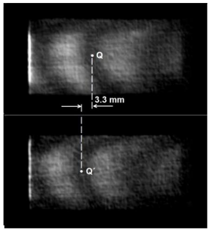
A plastic plate was excited by the LS vibrating at 80,0 Hz and was illuminated by the fringe pattern modulated by the FBE at 79,8 Hz. As expected, the fringe pattern moves back and forth which a frequency which comfortably allows determining its extreme positions. Figure 10 shows the two configurations of the fringe pattern with an average spatial period 10 mm. Point P is the extreme right position of the central fringe at a given instant, while P´ is its extreme left position. The distance between them is 3.3 mm, so that according to equation (7) the vibration amplitude is calculated to be a = 0.44. Figure 11 confirms the result obtained from Figure 10, showing the displacement undergone by a fringe pattern whose spatial period is ≈ 16 mm.
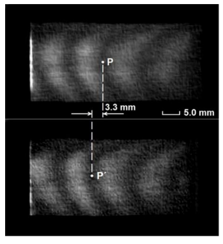
Figure 10 Vibration amplitude measurement by stroboscopy with a 10-mm spatial period interferogram: the distance between point P on the fringe pattern at his extreme right position (upper figure) and point P´ at the extreme left position (lower figure) is 3.3 mm.
The heterodyne measurement was much more feasible than the homodyne one due to our experimental conditions. The phase between the LS and the FBE outputs in our setup could only be controlled by steps, while the ideal way would be setting the phase continuously. These discrete phase steps cause interferogram jumps which sometimes may lose the reference and lead to ambiguous results. On the other hand, the heterodyne method allows that the fringes travel continuously with a speed that can be conveniently chosen by setting the FBE frequency.
The measurement procedure as described with Figures 10 and 11 is best suitable for the case in which all the points of the surface vibrate with the same amplitude. If the vibration map is not uniform, this procedure requires a larger manual effort, by repeating it in different points of the object. Other way for map determining, which is beyond the scope of this paper, consists in retrieving the phase map (by e.g. phase stepping methods) and the unwrapped phase of the object in the unperturbed and in the vibrating configuration. The amplitude map is obtained by subtracting both configurations. With this procedure the relative vibration phases can be also determined. The same arguments used in section 3.1 can be used to estimate the minimum measurable amplitude to be
6. Conclusions
This paper aims to demonstrate the feasibility of using structured light for vibration measurement. In this framework, the principles for vibration measurement based on fringe projection were proposed and discussed. It has been demonstrated the measurement of vibration amplitudes in the range of millimeters and tenths of millimeters, which is a range that usually cannot be easily performed by other whole-field techniques like time average holography and DSPI. The measurable frequency range is limited by the PZT-M and the FBE responsivities only. Some adjustments difficulties may eventually occur when the object vibration frequency matches the camera acquisition rate. This drawback can be overcome due to the fact that the fringes and the matching between the object frequency and the illumination frequency can be performed by directly observing the fringes on the surface, without the need of the camera. In this particular case the camera is useful just for image acquisition and storage.
Fringe projection techniques have the interesting feature to allow scaling the measurement sensitivity by conveniently adjusting the incidence angle. The use of the Twyman-Green interferometer is a very effective experimental solution, since it both produces the structured light and modulates the phase to make the interferogram oscillate. Moreover, it easily allows a convenient change of the spatial period. Differently from other whole-field methods, fringe pattern projection also allows the measurement of surfaces that vibrate as a whole, not requiring the existence of a nodal region. Nevertheless, the proposed method is also able to identify and evaluate regions with different vibration amplitudes, as demonstrated in Figure. 7.
Since some objects may vibrate at more than one frequency - the vibration harmonics - it is sometimes not possible to achieve a totally still fringe pattern by employing the phase modulation or stroboscopic techniques, because they are applicable to one frequency only. Hence, the visibility of resulting frozen interferogram may be lower than the visibility of the unexcited surface. It can be verified by carefully comparing Figures 5a and 5d. In some cases - depending on the exciting frequencies and intensities - static fringe patterns cannot be obtained at all.
For the present purpose, both the Twyman-Green and the Fabry-Perot interferometer can be constructed to be very compact and rugged, in order to operate in somewhat noisy environments without harmful instabilities; moreover, the relatively large measurable amplitudes does enable to perform vibration measurements of objects in such environments, without the requirement of placing them on damped table tops. Those features point out to applications of the technique to perform the testing of vibrating apparatuses and machines in industrial environments.
The way it was presented in this article, our technique is limited to analyze the vibration of flat or nearly flat surfaces only. The analysis of more complex surfaces would require a previous knowledge about its shape and/or an illumination scheme with more than one incidence angle. Those possibilities are currently under study.

