


 nueva página del texto (beta)
 Inglés (pdf)
 Artículo en XML
 Referencias del artículo
 Enviar artículo por email
 Citado por SciELO
  Similares en
SciELO
Similares en
SciELO 
 Permalink
1. Introduction
Transmitting compressed images over heterogeneous networks such as the Internet requires that the compression algorithm be quality and resolution scalable. A quality scalable image compression system creates a bit-stream in which the data is arranged in such a way that the bits that have the higher quality improvement are placed before the other bits. As such, the image can be decompressed at any bit rate while the (full-size) image quality is the best at this rate. In this way, a low bandwidth user can reconstruct a low-quality image while a user that has high bandwidth may reconstruct the image at high quality. On the other hand, a resolution scalable compression creates a bit-stream which consists of several subsets. The first subset contains the data that belong to the lowest resolution (size) image. The next subset (and all the next subsets) contains the necessary data that is required to reconstruct the image at a larger resolution. Therefore, if only the first subset is received, then the image can be reconstructed at the lowest size. If larger image size is desired, the decoder utilizes this subset and the next received subsets. Resolution scalability is useful for users that have diverse display resolutions, such as smartphones, tablets, laptops, desktop computers, and TV. Resolution scalability is also useful for image browsing. For image browsing, the user first receives a fingernail image (a small and rough approximation of the original image) that is ample for deciding if the image must be received fully or not. Just in case of needing the total size image, the user downloads the rest needed information. It is advantageous to combine both types of scalabilities to create a highly or full scalable bit-stream which is both resolution and quality scalable (Al-Janabi, 2019; Rüefenacht et al., 2019).
Scalability imposes an important restriction on the encoder. Specifically, it must operate without any earlier information about the quality and the size at which the image will be recovered by the users. Thus, the coder has to compress the image at full resolution and quality. After that, the compressed bit-stream is stored on a server. Users with various image quality and display resolution requirements send requests to the server, which delivers the appropriate scaled bit-stream to each one of them (Cappellari et al., 2011).
It is well known that the 2-dimensional discrete wavelet transform (2D-DWT) is an indispensable tool for the scalable compression of images. Its local spatiality feature simplifies quality scalability while its multi-resolution nature easily provides resolution scalability. Briefly, the forward 2D-DWT starts by decomposing the original image into four subbands referred to as LL1, HL1, LH1, and HH1. Next, the LL1 subband is also decomposed into another four subbands referred to as LL2, HL2, LH2, and HH2. The LLx subband may be decomposed M times resulting in 3M+1 subbands. At any decomposition stage, the LLm subband, m = 1,2 … M, represents a good approximation copy of the original image at reduced resolution with a size equal to 1/22m the original image size.
The inverse 2D-DWT starts by combining the LLM subband with the HLM, LHM,and HHM subbands to reconstruct the LLM-1 subband. The inverse process can be done up to M times to obtain a replica of the original image. Figure 1 shows the effect of the 2D-DWT on the test image "Camera Man" for two decomposition levels (M = 2). The first decomposition level splits the image into LL1, HL1, LH1, and HH1 subbands and the second level splits the LL1 subband into LL2, HL2, LH2, and HH2 subbands. As seen, the LL1 and the LL2 subbands are good approximated copies of the original image with sizes equal to 1/22 = 1/4 and to 1/24 = 1/16 the original image size respectively (Van Fleet, 2019; Vetterli, 2001).
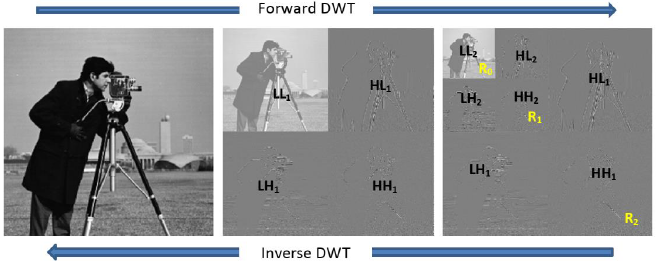
The wavelet subbands are arranged into M+1 resolution levels labeled R0, R1 … RM. The lowermost resolution level, R0, consists of the LLM subband only. Each o ne of the next levels Rm, 1 ≤ m ≤ M, consists of the three subbands HLM-m+1, LHM-m+1, and HHM-m+1 that are necessary to reconstruct the LLM-m subband during the inverse 2D-DWT process. Refer to Figure 1, the wavelet image has three resolution levels (R0, R1 and R2) that are represented by the yellow colour located at the down-right corner boundary of the corresponding resolution level. At the decoder, an image at the lowest resolution (1/16 the image size) can be obtained directly from the LL2 subband. The image may be recovered at higher resolution by combining the LL2 subband with the three subbands of R1 (HL2, LH2, and HH2), and performing one stage of inverse 2D-DWT to obtain LL1 (1/4 the image size). Finally, the image may be recovered at the biggest resolution (the entire image size) by combining the LL1 subband with the 3 subbands of R2 (HL1, LH1, and HH1), and carry out another stage of inverse 2D-DWT to get a replica of the original image. Therefore, a resolution scalable bit-stream can be easily achieved if the resolution levels are encoded successively and are identifiable within the compressed bit-stream (Taubman et al., 2002).
The set partitioning in hierarchical trees (SPIHT) (Said & Pearlman, 1996) is a powerful wavelet-based image compression algorithm. Its main pros are it has reasonable complexity, good PSNR (peak signal to noise ratio) vs. the bit rate performance, and it creates a quality scalable bit-stream. At its invention time, the last feature was very interesting as it adds freedom to the user to select the desired quality of the received image very easily. However, this feature is not sufficient nowadays for users that have devices with diverse display resolution capabilities such as laptops smartphones, tablet PCs, etc. As such, adding resolution scalability to SPIHT to generate a highly (rate and resolution) scalable bit-stream is very valuable (Cappellari et al., 2011; Wu et al., 2013). The second important weakness of SPIHT is its massive memory consumption, and complex memory management, which are caused by the use of three linked lists to save the image pixels’ coordinates. These lists consume memory about 2.5 times the DWT image (Chew et al., 2009; Singh & Butola, 2015) which represents a true constraint for low memory devices such as wireless sensors (Deepthi et al., 2018; ZainEldin et al., 2015) or for compressing volumetric medical images (Kamargaonkar & Sharma, 2016; Panjavamam & Bhuvaneswari, 2017). In addition, in the case of compressing multi-components images such as RGB colour images in parallel, the algorithm would need a memory of about 3x2.5 = 7.5 times the DWT image which represents a very serious obstacle. Finally, from the scalability point of view, using the linked lists prohibits resolution scalability due to the recurrent process of removing/adding pixels from/to lists, which makes the stored pixels in these lists not ordered according to the resolution levels (Cappellari et al., 2011; Taubman et al., 2002).
The SPIHT starts by applying the octave 2D-DWT to the image for M decomposition levels (normally M = 5). Next, every DWT coefficient c ij is quantized to
where cmax is the magnitude of the pixel that has the maximum value in the DWT image, and
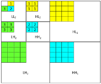
A closer look at Figure 1 reveals that there exists a shadow for the DWT image in all subbands. This means that if a coefficient located at a given position in the LLM subband is ISG, then the coefficients located at the other subbands that have the same position (with respect to their subbands), are also expected to be ISG. SPIHT exploits this feature to collect as many ISG coefficients as possible and coding them by one symbol. This is attained by combining these ISG coefficients together to build trees referred to as spatial orientation trees (SOTs). The primary roots of these SOTs are the pixels of the LLM subband excluding the top-left pixel in every set of (2×2) pixels. Every one of the three roots in each (2×2) set is considered a parent for four offspring located at HLM, LHM, and HHM respectively according to its orientation. That is, the top-right pixel is linked to HLM, the down-left pixel is linked to LHM, and the down-right pixel is linked to HHM. Then every pixel in subbands HLm, LHm, and HHm, M ≥ m ≥ 2, is considered a root (parent) to four offspring located at HLm-1, LHm-1, and Hm-1 respectively. Notice that the pixels in the HL1, LH1, and HH1 subbands have no offspring as they are the leaves of the trees. Figure 2 describes the SOTs of the first set of size (2×2) pixels in the subband LL2 for an image decomposed to two 2D-DWT levels, where each numbered colour represents a root of an entire SOT that extends across several resolution levels, and the unnumbered colour represent the leaves of these SOTs.
SPIHT utilizes three linked lists referred to as the list of insignificant pixels (LIP), the list of insignificant sets (LIS), and the list of significant pixels (LSP). The LIP and LSP keep the (i,j) coordinates of the ISG, and SG pixels respectively while the LIS keeps the (i,j) coordinates of the roots of the SOTs. SPIHT makes use of two type of roots. A root of type A represents the parent of a whole SOT, while a root of type B represents the parent of a partial SOT, which is a whole SOT excluding its four direct offspring (children). The LSP is initialized empty, the LIP is initialized by the (i,j) coordinates of the pixels in the LLM subband, and the LIS is initialized by the (i,j) coordinates of the primary parent roots of SOTs, which are the pixels in the LLM subband excluding the top-left pixel in every (2×2) set.
The first coding pass consists of the sorting sub-pass while the next coding passes consist of the sorting and the refinement sub-passes. Over the sorting sub-pass, every pixel cij in LIP is examined for the current threshold TH. If cij is ISG, a 0 is sent to the output bit-stream. If cij is SG, a 1 and its sign bit are sent to the bit-stream, and the pixel’s coordinates are transferred to LSP for refinement in the next passes. Next, each root rij in LIS is examined. if rij is of type A, its entire SOT is constructed and examined. If the SOT is still ISG, a 0 is sent to the bit-stream. Conversely, if the SOT is SG, then a 1 is sent to the bit-stream, and the four direct offspring of rij are examined. If an offspring is ISG, a 0 is sent to the bit-stream and its (i,j) coordinates are added to LIP to be tested in the next coding passes. If the offspring is SG, a 1, and its sign bit are sent to the bit-stream, and its (i,j) coordinates are added to LSP for refinement during the next passes. Finally, if rij is of type A and has grandchildren (i.e., it lies in LLM to HH2 subbands), then rij is removed from current position and added to the end of LIS as a type B root to be examined later on at the same pass. Alternatively, if rij is of type B, so a partial SOT that excludes its direct four offspring is constructed and examined again. If this partial SOT is SG, then a 1 is sent to the bit-stream, rij is removed from LIS, and each one of its four offspring is added to the end of LIS as a type A root to be examined later on at the same pass. If the partial SOT is ISG, then a 0 is sent to the bit-stream and rij is kept in LIS to be examined again in the following coding pass.
All pixels in LSP are refined during the refinement sub-pass, with the exception of those added during the current pass. A pixel cij is refined by sending its nth MSB to the bit-stream. After finishing the sorting and refinement sub-passes, the threshold TH is halved to begin a new coding pass. This process is repeated till the threshold is equal to 1, which means that all the pixels are encoded.
Several works interested in increasing the PSNR vs. the bit rate performance of SPIHT are presented cf. (Çekli & Akman, 2017; Çekli & Akman, 2019; Lee & Hung, 2018; Li & Liu, 2017; Sri & Sahu, 2019). The modified SPIHT (MSPIHT) algorithm presented by Rema et al. (2015) is one of the most efficient algorithms found in the literature. The MSPIHT algorithm used modified SOTs that ensure that the algorithm codes the more significant information in the initial bit-planes. It enhanced the PSNR at very low bit rates (less than 0.5 bpp) but gave approximately the same PSNR for bit rates greater than 0.5 bpp. Furthermore, MSPIHT has the same limitations as SPIHT regarding memory consumption and management. Al-Janabi (2013) proposed an efficient, low complexity, and low memory algorithm termed the Single List SPIHT (SLS). It reduced the memory consumption of SPIHT to about 80% by using one list of size equal to 1/4 the image size and two-state marker bits per pixel. At the same time, it preserved the PSNR and the low complexity features of SPIHT.
Danyali and Mertins (2004) focused on solving the scalability problem of SPIHT in their highly scalable-SPIHT (HS-SPIHT) algorithm. The HS-SPIHT algorithm added resolution scalability to SPIHT by utilizing resolution-dependent sorting passes with the related resolution-dependent linked lists. That is, for every resolution level Rm , m = 0, 1…M, a set of LIP, LSP, and LIS lists are employed. Therefore, there are LIPm, LSPm, and LISm. In each coding pass, the coder starts encoding from resolution level 0 and proceeds to the utmost level M. The algorithm first does the sorting sub-pass for the coefficients within the LIPm, and then it processes the roots in the LISm in the same way as done in SPIHT. In the refinement sub-pass, each pixel in LSPm is refined by sending its nth MSB to the bit-stream. After finishing the sorting and refinement sub-passes for resolution Rm, the process is repeated for the lists related to the subsequent resolution levels. Unfortunately, the HS-SPIHT algorithm has also the same weakness of SPIHT regarding memory consumption. Furthermore, it must deal with 3M linked lists instead of 3. This needs extra efforts for memory management and consequently increases the complexity of the algorithm as compared to the SPIHT algorithm.
Alam and Khan (2012) introduced the Listless HS-SPIHT (LHS-SPIHT) algorithm. It utilized the linear indexing technique to convert the DWT image from a 2D array to a 1D array of the same size to simplify the tracking of set partitioning. The functionalities of the lists LIPm, LSPm, and LISm of HS-SPIHT are performed using fixed-size state marker bits. That is, rather than adding the ISG pixels to LIPm, the SG pixels to LSPm, and the roots to LISm, the corresponding state marker bit is updated accordingly. For example, updating the marker bit of a pixel cij that lies in Rm to 1 is equivalent to adding its coordinates to LIPm. Consequently, rather than of examining the pixels in every LIPm only, the algorithm must examine the state marker bit of every pixel within the DWT image and codes the pixels that have a marker bit equals to 1 only. The same thing occurs for the SG pixels in every LSPm and the roots in every LISm. This means that LHS-SPIHT must examine all the image pixels twice, and must examine the roots in subbands LLM to HH2 once in each coding pass. As a result, the algorithm's complexity rises when compared to HS-SPIHT, and consequently the complexity rises even more when compared to SPIHT. The average memory of the state marker is 4 bits per pixel. Since each pixel in the DWT image is represented by 16 bits, so the marker bits need additional memory equal to 1/4 the size of the DWT image. More importantly, using the linear indexing technique necessitates either saving the 2D-DWT image into the main memory and then writing it into a 1D array or both 2D-DWT images and the 1D array must be available in memory at the same time. Unfortunately, the former solution is time-consuming while the latter one demands additional memory equals to the DWT image (Drozdek, 2012). So, the actual memory of LHS-SPIHT is equal to 1+1/4 = 1.25 the image size.
2. The proposed algorithms
This section first presents a modified version of the SPIHT algorithm termed the simplified SPIHT (SSPIHT) as it employs one type of roots instead of two. Then, the proposed Highly Scalable Listless SPIHT (HSLS) algorithm that represents the current work's main contribution is introduced. The proposed work reduces the memory of the SLS algorithm presented in (Al-Janabi, 2013) further by replacing the list with state marker bits that consume on average 0.5 bit per pixel. More importantly, it upgrades the SLS algorithm to creates a highly scalable bit-stream that can be decompressed at numerous bit rates and resolutions by processing the resolution levels in each coding pass incrementally. Finally, the Interleaved HSLS (IHSLS) which is a simplified version of HSLS is put forward.
2.1. The SSPIHT algorithm
Recall that in SPIHT, there are two types of roots. A root of type A is coded by constructing its complete SOT, and if this SOT is SG, and the root has grandchildren, then the root type is changed to type B root and added to LIS again. A type B root is coded by constructing its partial SOT (which excludes the four direct offspring of the root). And if this SOT is SG, then the root is taken out from LIS and its four direct offspring are added to LIS as type A roots. This means that for every root, the SOT must be constructed twice in each coding pass; one when the root is of type A, and one when it is transformed to type B. The proposed SSPIHT doesn’t need to use two types of roots. It is based on the observation that if a complete SOT of a given root is SG, then its partial SOT has a high probability of being SG too (Wenjun et al., 2002). Thus, the condition of adding its four direct offspring to LIS as roots of type A has a high chance of being satisfied. In other words, there is no need to do the condition test.
In SSPIHT, the coding of the LIP and LSP is done exactly as in SPIHT. However, the LIS is processed differently as follows: for every root in LIS, its whole SOT is constructed and examined for significance. If the SOT is ISG, a 0 is sent to the bit-stream as before. If the SOT is SG, then a 1 is sent to the bit-stream, and each one of the root’s four direct offspring is coded as done in SPIHT. Finally (and more importantly), if this SG root has grandchildren (i.e., it lies in LLM to HH2 subbands), then the root is taken out from LIS and each one of its four direct offspring is added as a root to the end of LIS to be examined later during the present pass. This modification avoids the extra processing time for constructing the partial SOT for every root of type B and eliminates the need of using the type bit. In addition, SSPIHT has superior PSNR performance than the MSPIHT algorithm presented by Rema et al. (2015) which is optimized to improve the PSNR at low compression bit rates as will be shown experimentally in the next section.
2.2. The HSLS algorithm
The proposed HSLS algorithm benefits from the multi-resolution characteristics of the 2D-DWT to generate a highly scalable bit-stream that can be decompressed at more than one rate (quality) and more than one resolution (size). Like the LHS-SPIHT algorithm (Alam & Khan, 2012), the proposed HSLS algorithm also makes use of state marker bits instead of the linked lists used by SPIHT. However, the HSLS has the following advantages over LHS-SPIHT:
It doesn’t use the linear indexing technique to avoid the complexity or the memory increment of this technique as clarified previously.
HSLS utilizes one marker bit termed ( of size 2 bits for every pixel in the DWT image, and two markers termed ( and ( of size 1 bit each for every root in the subbands LLM to HH2. Since the total size of these subbands is equal to 1/4 the size of the image, so every root marker needs on average 1/4 bit. So, the total memory consumed by our HSLS algorithm is 2+1/4+1/4 = 2.5 bits per pixel only. In contrast, LHS-SPIHT used an average of 4 bits per pixel (Alam & Khan, 2012).
Like SSPIHT, it employs one type of roots.
It eliminates the need to examine all the image pixels twice per pass. The main idea behind this is based on the fact that the pixels stored in the LIP represent the ISG offspring, and the pixels stored in the LSP represent the SG offspring of the roots of the SOTs that are found SG. So, these ISG and SG pixels can be easily deduced from the parent SG roots. In this way, the LIP and LSP can be dispensed by only computing the offspring that belong to the roots of the SG SOTs in each coding pass. Since these roots are located in subbands LLM to HH2 which have a size equal to 1/4 the DWT image size, and since only the SG SOTs are processed, then at most only 1/4 the image pixels need to be processed instead of testing all the image pixels two times in each pass as done in LHS- SPIHT (Alam & Khan, 2012). Evidently, this will reduce the algorithm's computational time.
The purpose of the state marker bits δ, α, and β is to indicate the significance status of the corresponding pixel and root as follows:
δij = 0: the pixel cij is ISG.
δij = 1: cij has just become SG in the current coding pass.
δij = 2: cij is found SG in one of the previous coding passes.
αij = 0: the root rij has an ISG SOT.
αij = 1: rij has a SG SOT.
βij = 0: rij is not considered for testing in the current coding pass or it is tested in a previous coding pass.
At initialization, HSLS computes the threshold TH using Eq. 1. Then, it sets the marker bit δ of every pixel in the DWT image to 0 to indicate that all the pixels are still ISG, sets the marker bit α for every root to 0 to indicate that all the roots are still ISG, and finally sets the marker bit β of every root in the LLM subband to 1, and all other roots to 0. Setting the marker bit βij of the root rij to 1 is equivalent to adding the (i,j) coordinates of rij to LIS in SPIHT.
The first bit-plane coding pass consists of the sorting sub-pass only while the other passes consist of the sorting and refinement sub-passes. To preserve resolution scalability in each coding pass, the algorithm scans the DWT image from the lowest resolution level R0, which contains the LLM subband only, to the utmost resolution level RM, which contains the HL1, LH1, and HH1 subbands. That is, in each coding pass, the algorithm performs the sorting sub-pass for all resolutions incrementally, and then performs the refinement sub-pass for all resolutions incrementally too.
The sorting sub-pass starts by coding each pixel cij in resolution R0 by the code_pixel(cij) procedure described next. Then, it will proceed to the next resolutions (R1 - RM). For every resolution Rm, 1 ≤ m ≤ M, all the parent roots are examined. It is worth noting that the parent roots of Rm lie in Rm-1 (i.e., the parent roots of R1 lie in R0 and so on). So, in fact, the parent roots are located in (R0 - RM-1). So, for every resolution, Rm, 0 ≤ m ≤ M -1, each root rij that is found SG in a previous coding pass (i.e., with αij = 1) is processed by computing its direct four offspring Ok, K = 1,2,3,4. Then, each offspring Ok is coded as a pixel by the code_pixel(Ok). Notice that this step is left out in the first coding pass as all the roots are still ISG. Finally, for every resolution, Rm, 0 ≤ m ≤ M-1, each root rij that is considered for testing in the current coding pass (i.e., with βij = 1), its SOT is constructed and tested for significance. If rij has still an ISG SOT, a 0 is transmitted to the bit-stream, and rij will be examined again in the next pass. If rij has an SG SOT, a 1 is sent to the bit-stream, αij is updated to 1 (i.e., rij is marked as a SG root), and βij is updated back to 0 (this is equivalent to removing the (i,j) coordinates of rij from LIS). Then, each one of the rij’s direct four offspring Ok, k = 1, 2, 3, 4 is coded as a pixel by the code_pixel(Ok). Finally, the marker bit of each one of its direct four offspring
The refinement sub-pass firstly sends every pixel cij in R0 that is found SG in the previous passes (i.e., with δij = 2) to the refine_pixel(cij) procedure, described shortly, for refining. Next, for every resolution level Rm, 1 ≤ m ≤ M, each one of its SG roots rij (i.e., with αij=1) that lie in Rm-1, its direct four offspring Ok, k = 1,2,3,4 is coded by the refine_pixel(Ok) procedure to refine its magnitude. Lastly, the threshold TH is updated to TH/2 to proceed to the next coding pass until the threshold is equal to 1 indicating that all the pixels are encoded.
The code_pixel(cij) procedure works as follows: If cij is yet marked ISG (i.e., δij = 0), cij is tested for significance. If
In the refine_pixel(cij) procedure, if
The pseudocodes of the encoder and decoder of the proposed HSLS are shown in Figure 3a and 3b respectively. The following remarks clarify the operation of the algorithm.
As mentioned previously, the scalable encoder has to encode the image at the full bit rate (i.e., until TH = 1). On the other hand, the decoder may stop when the target bit rate is reached.
As mentioned before, for a highly scalable bit-stream, each resolution level within each coding pass must be recognizable in the bit-stream. This is easily attained since these levels are encoded incrementally in each coding pass, by adding a marker at the beginning of each resolution level, that designates the length of corresponding the level.
The decoder algorithm executes the same four steps of the encoder. The difference is that the decoder works inversely. That is, when it receives 0/1, this indicates that the corresponding pixel or SOT is ISG/SG respectively. Then, the decoder follows the same route as the encoder. Notice that if a pixel cij is SG, the decoder recognizes that the magnitude of cij is in the range [TH ( 2TH), so cij is reconstructed at the midpoint which is equal to ±1.5(TH based on its sign bit. Then every received refinement bit increases the precision of the pixel by ±TH/2 according to the received bit and the sign of the pixel. For example, assume that at the encoder the initial threshold TH = 16 and cij = +19. cij is SG as +19 ≥ 16. So, at pass#1, the encoder sends 1 and the sign bit 0, and it updates cij to 19-16 = 3. At pass#2, the encoder updates TH to TH/2 = 8, and sends 0 as 3 < 8. At pass#3, it updates TH to 4, and sends 0 since 3 < 4. Finally, at pass#4, it updates TH to 2 and sends 1 since 3 ≥ 2. The decoder first receives TH = 16. At pass#1, the received bits are 1 and 0, so it reconstructs cij to +1.5×TH = +1.5×16 = +24. At pass#2, TH is updated to 8 and the received bit = 0, so cij is updated to +24-4 = +20. At pass#3, TH = 4 and the received bit = 0, then cij is set to +20-2 = +18. Finally, at pass#4, TH = 2 and the received bit = 1, then cij is updated to +18 +1 = +19 which is equal to the original value.
The decoder can reconstruct an image at resolution Rm, 0 ≤ m ≤ M by receiving the data that corresponds to R0 to Rm and bypassing the data of the other resolutions in each coding pass. Then it performs m stages of inverse 2D-DWT only to recover the image with size equal to

2.3. The IHSLS algorithm
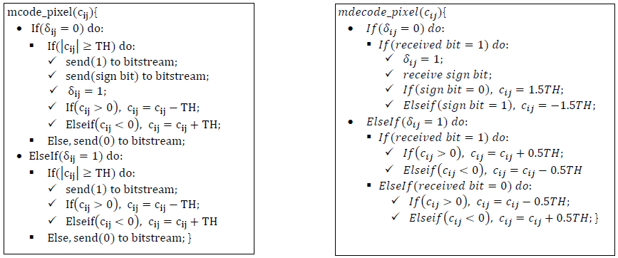
The IHSLS algorithm has only one coding pass per bit-plane instead of two. The new coding pass is termed the merging pass. It merges the sorting sub-pass with the refinement sub-pass. However, the code_pixel(cij) is modified to code the pixels that are still ISG and to refine the pixels that became SG in the preceding coding passes. The merged mcode_pixel(cij) starts by examining the pixel’s status bit δij. If δij = 0 (i.e., cij is yet untested), then cij is examined for significance and coded exactly as done in the code_pixel(cij). On the other hand, if δij = 1 (i.e., cij is found SG at a previous pass), then cij is refined as given in the refine_pixel(cij). Notice that in the adopted coding method, the pixel may be either SG or ISG. Therefore, one marker bit for δ is sufficient: δij = 0 if cij is ISG, and δij = 1 if cij is SG. The pseudocodes of the merged mcode_pixel(cij) and the merged mdecode_pixel(cij) procedures are shown in Figure 4. The same notes of the decoding procedure explained previously apply to mdecode_pixel(cij).
Compared to the HSLS algorithm, the IHSLS algorithm runs slightly faster because it performs one coding pass per bit-plane instead of two. In addition, it has a slightly lower memory requirement as it uses one bit for δ instead of two. So, the total memory of IHSLS is 1.5 bits per pixel instead of the 2.5 bits per pixel that are required by HSLS. However, the cost of these benefits is a slight decrement in PSNR performance as compared to that of HSLS due to the coding pass merging
3. Results and analysis
The proposed algorithms are implemented using Borland C++ v. 5.02 under Intel μprocessor Core i3 PC with 1.8 GHz CPU, and 2 GB RAM. The popular grayscale test images "Lena," "Barbara," "Goldhill," and "Mandrill" of size (512×512) pixels are used in the simulation. As with other algorithms, the image is transformed by the octave 2D-DWT with 5 decomposition levels using the CDF 9/7 wavelet filter (Vetterli, 2001). The PSNR of the algorithm vs. the bit rate, as well as its computational time vs. the bit rate, are used to represent the results. The bit rate is the average number of bits per pixel (bpp) of the compressed image. The PSNR measures how similar the original and recovered images are. It is defined as (Al-Janabi, 2015):
Where pmax is the maximum pixel value in the original image (pmax = 28 = 255) (for grayscale images), and MSE is the mean-squared error between the original image Io and the recovered image Ir, given by:
where MN is the image size (the number of image pixels). Obviously, for any bit rate, a higher PSNR value is preferred.
3.1. Performance of the proposed SSPIHT algorithm
Table 1 depicts the PSNR vs. bit rate for the proposed SSPIHT, the original SPIHT, and the MSPIHT algorithm (Rema et al., 2015) which is optimized to improve the PSNR at low bit rates. The PSNR of our SSPIHT algorithm is boldfaced where it is higher than that of MSPIHT. As it is clearly shown, the PSNR of SSPIHT is higher for nearly all images at all bit rates. This means that our SSPIHT performs better than SPIHT and MSPIHT. In addition, as will be seen in the next section, the proposed SSPIHT runs faster than the original SPIHT, and therefore it runs also faster than MSPIHT since the latter two algorithms have nearly the same complexity (Rema et al., 2015). Figure 5 shows the original “Lena” image and the decoded ones at several bit rates using SSPIHT
Table 1 PSNR vs. bit rate for the proposed SSPIHT, SPIHT, and MSPIHT algorithms.
| Bit rate (bpp) |
PSNR (dB) | ||||||||
|---|---|---|---|---|---|---|---|---|---|
| Lena 512×512 | Goldhill 512×512 | Barbara 512×512 | |||||||
| SPIHT | MSPIHT | Proposed SSPIHT |
SPIHT | MSPIHT | Proposed SSPIHT |
SPIHT | MSPIHT | Proposed SSPIHT |
|
| 0.01 | 11.88 | 15.31 | 21.02 | 11.32 | 16.32 | 21.87 | 11.56 | 15.29 | 19.89 |
| 0.03 | 22.31 | 23.69 | 23.44 | 21.99 | 23.07 | 23.65 | 20.34 | 21.15 | 21.58 |
| 0.05 | 25.03 | 25.70 | 26.49 | 24.17 | 24.66 | 25.60 | 21.92 | 22.18 | 22.88 |
| 0.1 | 28.44 | 28.68 | 28.88 | 26.30 | 26.51 | 27.13 | 23.39 | 23.55 | 24.24 |
| 0.2 | 31.74 | 31.88 | 31.94 | 28.40 | 28.50 | 29.16 | 25.64 | 25.83 | 26.34 |
| 0.5 | 36.46 | 36.52 | 36.27 | 31.47 | 31.52 | 32.30 | 30.38 | 30.46 | 31.11 |

3.2. Performance results of the highly scalable algorithms with full resolution images
Tables 2 and 3 give a comparison of the PSNR vs. the bit rate of the proposed HSLS and IHSLS algorithms with the highly scalable algorithms HS-SPIHT (Danyali & Mertins, 2004) and LHS-SPIHT (Alam & Khan, 2012) at full resolution (size) image. Firstly, it should be noted that the PSNR of HS-SPIHT is higher than that of LHS-SPIHT and the proposed algorithms. This is normal due to removing the lists from LHS-SPIHT and from our algorithms. In other words, the slight PSNR decrement is the price of the huge reduction in computer memory resources.
Table 2 PSNR vs. bit rate for Lena and Barbara images.
| Bit rate (bpp) |
PSNR (dB) | |||||||
|---|---|---|---|---|---|---|---|---|
| Lena 512×512 | Barbara 512(512 | |||||||
| HS- SPIHT |
LHS- SPIHT |
Proposed HSLS |
Proposed IHSLS |
HS- SPIHT |
LHS- SPIHT |
Proposed HSLS |
Proposed IHSLS |
|
| 0.0625 | 27.52 | 26.85 | 27.35 | 27.28 | 22.97 | 22.59 | 23.37 | 23.30 |
| 0.125 | 30.31 | 29.93 | 30.04 | 29.86 | 24.12 | 23.65 | 24.26 | 24.30 |
| 0.25 | 33.33 | 33.19 | 33.00 | 32.83 | 26.68 | 26.75 | 27.31 | 27.01 |
| 0.5 | 36.57 | 36.49 | 36.24 | 36.08 | 30.53 | 30.48 | 31.05 | 30.83 |
| 1 | 39.93 | 39.58 | 39.58 | 39.37 | 35.28 | 35.19 | 36.23 | 35.77 |
Table 3 PSNR vs. bit rate for Goldhill and Mandrill images.
| Bit rate (bpp) |
PSNR (dB) | |||||||
|---|---|---|---|---|---|---|---|---|
| Goldhill 512×512 | Mandrill 512×512 | |||||||
| HS- SPIHT |
LHS- SPIHT |
Proposed HSLS |
Proposed IHSLS |
HS- SPIHT |
LHS- SPIHT |
Proposed HSLS |
Proposed IHSLS |
|
| 0.0625 | 26.27 | 26.26 | 26.15 | 26.11 | 20.19 | 20.38 | 20.26 | 20.28 |
| 0.125 | 28.02 | 27.50 | 27.80 | 27.70 | 21.45 | 21.25 | 21.27 | 21.26 |
| 0.25 | 30.19 | 29.39 | 29.73 | 29.80 | 22.86 | 22.66 | 22.58 | 22.60 |
| 0.5 | 32.40 | 32.10 | 32.05 | 32.13 | 24.19 | 24.60 | 24.68 | 24.64 |
| 1 | 35.67 | 35.54 | 35.40 | 35.34 | 28.50 | 28.30 | 28.30 | 28.00 |
Secondly, the comparison will be between the LHS-SPIHT and the proposed HSLS and IHSLS algorithms since they don’t use lists. The PSNR of our HSLS and IHSLS algorithms is boldfaced where it is higher than that of LHS-SPIHT. As it can be seen, for the proposed HSLS, the PSNR is mostly higher for nearly all images at all bit rates. This means that the proposed HSLS is on par with the other algorithms in terms of performance. The advantages of the proposed algorithm are its lower memory (2.5 bits per pixel while the LHS-SPIHT needs 4 bits per pixel) as depicted previously, and its lower computational time as demonstrated within the next section. Finally, the PSNR of the IHSLS is slightly lower than that of the HSLS. This result is expected as a price for its speed enhancement due to using of one pass per bit-plane instead of two, and as a cost for its memory reduction (1.5 bits per pixel instead of 2.5 bits per pixel). However, it’s also competitive with the other algorithms.
3.3. Computational time calculation
Table 4 shows the encoding and decoding times of the algorithms measured in milliseconds (msec) vs. bit rate for the "Lena" image at full resolution.
Table 4 The encoding and decoding times vs. bit rate for Lena image.
| Bit rate (bpp) |
Encoding Time (msec) | Decoding Time (msec) | ||||||||
|---|---|---|---|---|---|---|---|---|---|---|
| SPIHT | SSPIHT | LHS- SPIHT |
HSLS | IHSLS | SPIHT | SSPIHT | LHS- SPIHT |
HSLS | IHSLS | |
| 0.125 | 15 | 12 | 24 | 16 | 14 | 5 | 5 | 11 | 7 | 5 |
| 0.25 | 20 | 16 | 28 | 22 | 18 | 10 | 10 | 17 | 12 | 10 |
| 0.5 | 26 | 23 | 33 | 26 | 24 | 20 | 20 | 28 | 23 | 21 |
| 1 | 31 | 28 | 38 | 31 | 28 | 25 | 25 | 33 | 27 | 26 |
| 2 | 63 | 60 | 52 | 64 | 60 | 32 | 32 | 45 | 35 | 33 |
The following observations can be deduced:
For any algorithm, its decoding time is shorter than its encoding time. This is normal for set partitioning algorithms as the decoder does not need to scan and process the pixels and sets to see if they are SG or not.
The proposed SSPIHT runs faster than the original SPIHT for all bit rates. This is due to eliminating the necessity to construct the SOTs twice in each coding pass.
The LHS-SPIHT, which creates a highly scalable bit-stream, runs about two times slower than the SPIHT since it needs to scan and examine all the image pixels two times per coding pass.
The proposed HSLS, which also creates a highly scalable bit-stream, has very little increment in the encoding and decoding times as compared to SSPIHT. This is because that the HSLS needs only to separate and identify the resolution levels.
Additionally, the HSLS, and SPIHT algorithms have approximately the same processing time. This means that our HSLS added resolution scalability, and reduced the memory requirements of SPIHT without paying any noticeable cost. In contrast, the HS-SPIHT increased the memory requirements, and increased the memory management, while the LHS-SPIHT increased the complexity further against SPIHT.
As expected, the Proposed IHSLS runs faster than HSLS due to pass merging
3.4. Performance results of the highly scalable algorithms at reduced resolution
A highly scalable decoder may reconstruct the image at a resolution less than that of the original image. Eqs. 2 and 3 can't be used to compute the PSNR in this case because the original and recovered images aren't the same size. Therefore, to be able to give numerical results at reduced resolution, the same manner used in (Danyali & Mertins, 2004) which is also used by Alam and Khan, (2012) will be employed. It utilizes the fact that an image with resolution s, 0 ≤ s ≤ M, is the subband LLM-S within the DWT image. So, the original LLM-S and the recovered LLM-S subbands are compared in place of the original and recovered images. For this case, pmax would become the maximum pixel value in the subband LLM-S. It can be shown that for a grayscale image (with 8 bpp), pmax is equal to (255 × 2M-s) (Danyali & Mertins, 2004). For instance, if an image with (512 × 512) pixels is decomposed with M = 5 wavelet levels, and the image is recovered at resolution s = 4, then LLM-s = LL5-4 = LL1 represents the recovered image which has (256 × 256) pixels (1/4 the original image size), and pmax = 255 × 25-4 = 510.
Tables 5 and 6 depict the PSNR vs. bit rate for the images at s = 4 (1/4 resolution), while Tables 7 and 8 depict the PSNR vs. bit rate for the images at s = 3 (1/16 resolution). The bit rates are computed using to the number of pixels in the full-size image. The PSNR of our HSLS and IHSLS algorithms is boldfaced where it is higher than that of LHS-SPIHT. It is worth to note that in Tables 7 and 8, the PSNR of our algorithms in the last row represents the PSNR achieved at full bit rate compression (i.e., the maximum achievable PSNR). For instance, for the “Lena” image, the proposed HSLS achieves PSNR = 64.77 dB @0.45 bpp. Evidently, at this full bit rate (0.45 bpp), the PSNR will be smaller than that of the other algorithms which calculated the PSNR @0.5 bpp. However, any PSNR higher than 50 dB is considered perfect in terms of image quality (Gu et al., 2013). As it can be seen, for “Barbara” and “Mandrill” images (which have more details than “Lena” and “Goldhill” images), the proposed HSLS performs better than the LHS-SPIHT and the HS-SPIHT for all bit rates. For “Lena” and “Goldhill” images, the PSNR of HSLS, LHS-SPIHT, and HS-SPIHT are very comparable. In addition, the proposed IHSLS has also a slightly lower PSNR than that of HSLS due to the adopted simplifications. On the other hand, it is superior to LHS-SPIHT and HS-SPIHT for “Barbara” and “Mandrill” images at all bit rates (except for “Mandrill” @0.5 bpp for s = 4, and @0.125 bpp for s = 3). Finally, for “Lena” and “Goldhill” images, the IHSLS is also very comparable to the LHS-SPIHT, and HS-SPIHT algorithms. This suggests that our algorithms are very successful for users that need to recover low-resolution images, such as that smartphones, tablets, etc.
Table 5 The PSNR vs. Bit rate for Lena and Barbara images @1/4 resolution (s = 4).
| Bit rate (bpp) |
PSNR (dB) | |||||||
|---|---|---|---|---|---|---|---|---|
| Lena | Barbara | |||||||
| HS- SPIHT |
LHS- SPIHT |
Proposed HSLS |
Proposed IHSLS |
HS- SPIHT |
LHS- SPIHT |
Proposed HSLS |
Proposed IHSLS |
|
| 0.0625 | 28.78 | 27.98 | 28.45 | 28.40 | 25.94 | 25.48 | 26.84 | 26.73 |
| 0.125 | 32.34 | 31.84 | 32.14 | 31.90 | 28.41 | 27.93 | 29.24 | 29.20 |
| 0.25 | 37.44 | 37.21 | 37.01 | 36.94 | 32.64 | 32.42 | 33.66 | 33.65 |
| 0.5 | 43.82 | 43.52 | 43.35 | 43.29 | 39.19 | 38.97 | 39.23 | 39.19 |
| 1 | 53.25 | 53.17 | 53.05 | 52.92 | 50.12 | 50.02 | 50.19 | 50.17 |
Table 6 The PSNR vs. Bit rate for Goldhill and Mandrill images @1/4 resolution (s = 4).
| Bit rate (bpp) |
PSNR (dB) | |||||||
|---|---|---|---|---|---|---|---|---|
| Goldhill | Mandrill | |||||||
| HS- SPIHT |
LHS- SPIHT |
Proposed HSLS |
Proposed IHSLS |
HS- SPIHT |
LHS- SPIHT |
Proposed HSLS |
Proposed IHSLS |
|
| 0.0625 | 27.79 | 27.36 | 27.61 | 27.59 | 21.47 | 21.28 | 22.74 | 22.83 |
| 0.125 | 30.81 | 29.78 | 30.21 | 30.03 | 23.65 | 23.45 | 24.73 | 24.42 |
| 0.25 | 33.86 | 32.97 | 32.79 | 32.87 | 28.79 | 28.59 | 28.87 | 28.75 |
| 0.5 | 38.81 | 38.51 | 38.62 | 38.59 | 31.41 | 31.21 | 31.58 | 30.95 |
| 1 | 49.97 | 49.73 | 49.77 | 49.76 | 39.42 | 39.23 | 39.52 | 39.48 |
Table 7 The PSNR vs. Bit rate for Lena and Barbara images @1/16 resolution (s = 3).
| Bit rate (bpp) |
PSNR (dB) | |||||||
|---|---|---|---|---|---|---|---|---|
| Lena | Barbara | |||||||
| HS- SPIHT |
LHS- SPIHT |
Proposed HSLS |
Proposed IHSLS |
HS- SPIHT |
LHS- SPIHT |
Proposed HSLS |
Proposed IHSLS |
|
| 0.0625 | 32.38 | 31.86 | 32.08 | 32.05 | 30.83 | 29.89 | 31.93 | 31.93 |
| 0.125 | 40.03 | 39.53 | 40.34 | 40.28 | 36.55 | 35.83 | 36.03 | 35.75 |
| 0.25 | 50.73 | 50.30 | 50.89 | 50.63 | 47.34 | 46.12 | 46.52 | 46.28 |
| 0.5 | 70.52 | 70.51 | 64.77 @0.45 bpp |
64.75 @0.45 bpp |
71.16 | 70.89 | 63.75 @0.46 bpp |
63.70 @0.46 bpp |
Table 8 The PSNR vs. Bit rate for Goldhill and Mandrill images @1/16 resolution (s = 3).
| Bit rate (bpp) |
PSNR (dB) | |||||||
|---|---|---|---|---|---|---|---|---|
| Goldhill | Mandrill | |||||||
| HS- SPIHT |
LHS- SPIHT |
Proposed HSLS |
Proposed IHSLS |
HS- SPIHT |
LHS- SPIHT |
Proposed HSLS |
Proposed IHSLS |
|
| 0.0625 | 31.48 | 30.86 | 31.33 | 31.28 | 25.40 | 25.21 | 26.00 | 26.13 |
| 0.125 | 37.13 | 36.12 | 36.87 | 36.82 | 31.49 | 31.31 | 30.42 | 30.62 |
| 0.25 | 47.96 | 46.87 | 47.05 | 46.95 | 40.98 | 40.82 | 40.87 | 40.87 |
| 0.5 | 70.91 | 70.71 | 64.80 @0.48 bpp |
64.80 @0.48 bpp |
60.05 | 59.97 | 64.77 @0.52 bpp |
64.77 @0.52 bpp |
4. Conclusions
In this paper, we presented a framework of three related scalable image compression algorithms. As demonstrated within the last section, the SSPIHT algorithm has lower complexity and improved performance than that of the original SPIHT. Additionally, at low bit rates, it provided higher PSNR than that of the MSPIHT algorithm, which is optimized for that purpose. The HSLS algorithm solved the dual problems of SPIHT: the scalability and the massive memory resources without paying any noticeable cost concerning its performance and complexity. In contrast, the HS-SPIHT increased the complexity and the memory while the LHS-SPIHT widely increased the complexity as compared to SPIHT. Moreover, our HSLS algorithm performed better than these algorithms when the image is recovered at reduced resolutions. Finally, the IHSLS algorithm is faster and consumes less memory than that of HSLS. As shown, the only price for these additional advantages is the very slight reduction in PSNR.
Conflict of interest
The authors do not have any type of conflict of interest to declare.
Financing
The authors did not receive any sponsorship to carry out the research reported in the present manuscript.

