


 nueva página del texto (beta)
 Inglés (pdf)
 Artículo en XML
 Referencias del artículo
 Enviar artículo por email
 Citado por SciELO
  Similares en
SciELO
Similares en
SciELO 
 Permalink
1. Introduction
The pH neutralization setup is widely used in the pH treatment of wastewater or runoff water from pharmaceutical or biotech organizations and construction sites (Aparna, 2014). By and large, the pH neutralization process plays a significant role in several industries, as it is necessary to neutralize the pH of the industrial fluid wastes before they are discharged into the atmosphere. The principal purpose of controlling a pH neutralization system is to maintain the pH value of the discharged effluent as per the environmental safety regulation of 6 to 8. A highly acidic or alkaline pH would be fatal to the ecological surroundings. However, control of a pH neutralization system is highly challenging and complicated because of the inherent nonlinearity in the system (Abdullah et al., 2012; Bharathi et al., 2007; Ibrahim & Murray-Smith, 2007; Saji & Sasi, 2011; Shinskey, 1973). Classical control methods prove to be beneficial only for linear processes and for analytical testing. For real-time control, the performance of the designed controller should be able to bypass the effects of nonlinearities, modeling errors and uncertainties, dead time, interaction effect, and dynamic behavior in the pH neutralization process (Bequette, 1991; Faanes & Skogestad, 2004).
The most widely used controller for this type of system is continuous Proportional-Integral-Derivative (PID) control, and experiments and studies have been carried out to figure out the appropriate tuning method for the PID controller. Saji and Sasi (2011) employed particle swarm optimization and Ant colony optimization algorithm to tune the PID controller parameters. They achieved setpoint tracking, robustness, and sensitivity from their nonlinear controller (Saji & Sasi, 2011). Bingi et al. (2016) preferred particle swarm optimization algorithm over Ziegler Nichols method to tune PID controller for a pH neutralization plant (Bingi et al., 2016). Tadeo et al. (2000) used a loop shaping approach by combining robust and graphical loop shaping to achieve robustness and reduce the effect of model uncertainty in the controller performance (Tadeo et al., 2000). Shabani et al. (2010) employed quantitative feedback theory-based controller to attain setpoint tracking and disturbance rejection despite inherent model uncertainties (Shabani et al., 2010). Ali (2001) compared the performance of a standard PI controller with a globally linearizing control algorithm and gain scheduling strategy in effectively controlling a complex pH process over a wide range of operating conditions without constant retuning (Ali, 2001).
In another work, Bingi et al. (2018, 2020) designed a setpoint weighted fractional-order PID tuned using an accelerated particle swarm optimization algorithm to achieve superior setpoint tracking in a pH neutralization plant (Bingi et al., 2018, 2020).
To assuage this need for effective control of the pH neutralization system and achieve desired disturbance rejection, setpoint tracking, sensitivity, and robustness, several optimizations, self-tuning, intelligent, robust, and model-based approaches have been proposed (Barve & Nataraj, 1999; Ibrahim, 2010; Moore, 1995).
In this paper, sections 2 and 3 describe the pH neutralization setup and its mathematical model and analysis. Section 4 explains the various tuning algorithms adopted to design the controller, and sections 5 and 6 present and analyze the response of the controlled system with different tuning algorithms in simulation. Section 7 describes the real-time implementation of the controllers in the system. Section 8 presents the experimental results; finally, the suitable controller for the proposed process based on the simulation and experimental results is deduced.
2. pH neutralization system
The pH neutralization process controls or maintains the pH of a solution such that it remains a neutral solution.
The solution whose pH is to be monitored is fed into the water tank at the top. This solution from the water tank is supplied to the process tank through a solenoid valve (SV). Depending on the initial pH value of the solution and based on whether the solution is to be neutralized or made acidic/alkaline, alkaline (0.1 N Sodium Hydroxide solution) and acidic solution (0.1 N Hydrochloric acid solution) are added to the process tank through Pump 1 & 2. A stirrer mixes the contents of the process tank before its pH is measured. The pH probe and transmitter measure the pH value of the solution in the process tank and convert it into (0-5) V range. The measured pH value is the controller input, and the controller varies the strokes per minute of the pumps, changing the inflow of acidic and alkaline solution to the process tank based on the desired pH value to be maintained in the process tank. Once the pH value is controlled or retained at the desired value, the contents of the process tank are emptied into the collecting container. Three hand valves, HV1, HV2, and HV3, are provided to drain the contents of the alkaline tank, collecting tank, and acid tank, respectively. Figure 1 portrays the schematic diagram of the pH neutralization setup.

The pH system is a Two-Input One-Output (TISO) system, where the concentration of the non-reacting acid solution and alkaline solution in the tanks (xca, xcb) are the states and pH of the solution is the controlled variable of the system. Pumps 1 and 2 act as the final control elements and strokes per minute (SPM) of pumps 1 and 2, and inflow rates of acid and alkaline solutions to the reactor tank (Fwa and Fwb) are the variables manipulated by the controller.
3. Empirical modeling
3.1. System modeling
The general representation of a pH system is given by (Alina & Madalina, 2016; Bharathi et al., 2007; Biagiola et al., 2016; Darab et al., 2012; Elameen et al., 2014; Rodriguez & Loparo, 2004),
State-space models derived from the above equations are,
The various parameters of the process were assumed, as stated in the following Table 1,
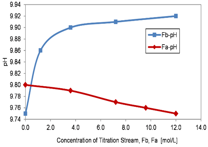
Depending on the required pH value from the process, either the acid solution or alkaline solution was added to the process tank. For instance, if the process solution is acidic, an alkaline solution was added to neutralize it and vice versa. State-space models for both the cases, stated in Eqs. 4 to 8, were derived from Eqs. 1 to 3. Then the various operating points obtained from the open-loop I/O characteristics (Table 2) were substituted to compute the state-space model and the corresponding transfer function, as shown in Table 3. Open-loop I/O characteristics from the process (Figure 2) were noted by varying one manipulated variable and maintaining the other variable constant. Initially, the inflow rate of the acidic solution was maintained at a constant value (Fwa = 7.2 L/h). Then, for various inflow rates of the alkaline solution (Fwb), the pH value of the solution in the process tank was recorded. Similarly, Fwb was maintained constant, and Fwa was varied, and the corresponding pH value was recorded.
Table 1 Operating data for the pH process.
| Parameter | Description | Value |
| R | The radius of the process tank | 8 cm |
| H | The maximum height of the process tank | 20 cm |
| C | The capacity of the process tank | 4.02 L |
| Coa, Cob | The concentration of acid and alkaline solution | 0.1 N |
| Fwa, Fwb | The flow rate of acid and alkaline solution to the process tank | 12 L/h |
| Ew | The equilibrium constant for water dissociation | 10-14 |
| xca, xcb | The concentration of the non-reacting acid solution and alkaline solution in tanks |
Table 2 Operating points obtained from I/O characteristics.
| Case | Operating Points |
| Case 1 Fwb Vs. pH |
Fwas = 7.2 L/h Fwbs = 7.2 L/h C = 4.02 L Cobs = 1.23*10-10 mol/L pHs = 9.91 |
| Case 2 Fwa Vs. pH |
Fwas = 7.2
L/h Fwbs = 7.2 L/h C = 4.02 L Coas = 1.7*10-10 mol/L pHs = 9.77 |
Table 3 State-space and transfer function model of the system.
| Case | State Space Model | Transfer Function |
| Fwb Vs. pH |
A = B = C = D = |
|
| Fwa Vs. pH |
A = B = C = D = |
|
From Table 3, it can be seen that, mathematically, the state space and transfer function model of both the cases are similar. Therefore, either case can represent the pH neutralization system in simulation.
3.3. Stability analysis
Eigenvalues and frequency response of the system were used to analyze the system’s stability. The system was completely stable since all its eigenvalues were negative, and the phase margin and the gain margin were positive values. Furthermore, the phase margin was higher than the gain margin, as stated in Table 4.
4. Controller tuning methods
For the proposed system, the PID controller was implemented to maintain the pH at a desired acidic, alkaline, or neutral value. Three tuning algorithms, a classic optimization algorithm, genetic algorithm (GA), a metaheuristic optimization algorithm, Bacterial Foraging Technique based Particle Swarm Optimization algorithm (BFTPSO), and a robust technique, quantitative feedback theory (QFT), were chosen to tune the PID controller for this nonlinear process.
4.1. Genetic algorithm
A population of solutions is continuously evolved in a genetic algorithm by modifying the bits of the solution based on a fitness function to obtain the optimal output from the optimization problem. The three most common operators for evolving the population of solutions are Selection, Crossover, and Mutation.
A standard genetic algorithm involves the following steps,
Step 1-Generation of an initial population of ‘n’ chromosomes.
Step 2-Calculation of the fitness function f(x) for each chromosome (x) in the population.
Step 3-Repetition of the following steps’ i’, ‘j,’ and ‘k’ until ‘n’ offspring are generated from ‘n’ chromosomes,
i) Creation of a fitting parent population depending on higher/lower fitness function value.
Usually, two-parent chromosomes are selected to apply other GA operators to it. However, in elitism selection, one best parent chromosome is kept until the next generation. Also, a parent chromosome may not be selected at all, or it may be selected more than once based on its fitness value.
j) Generation of several offspring at randomly chosen points of the parent population based on the crossover rate. Crossover facilitates the offspring to inherit unique features and the common features of the parent chromosomes.
k) Mutation of the offspring at randomly chosen points depending on the mutation probability. If the mutation probability is greater than the mutated chromosome, then the mutated is used in the new population. Else it is discarded.
Step 4-Replacement of the existing population with the newly created population.
Step 5-Repetition from Step 2 again.
In this work, Integral Time Weighted Absolute Error (ITAE) was regarded as the optimization function for the algorithm, and the controller parameters were computed for the most minimal ITAE value. One iteration completed one generation of the algorithm, and optimization was carried out for several generations until suitable controller gains that reduced the error in the system were attained. Sensitivity analysis was done for different population sizes, crossover, and mutation probabilities. The best results for this system were obtained in 300 iterations for a single-point crossover method with a probability of 0.2 and with a uniform mutation probability of 0.05. An initial population size of 100 and a combination of elitism and stochastic uniform selection methods were employed to implement the algorithm.
4.2. Bacterial foraging technique-based particle swarm optimization algorithm
Bacterial Foraging Technique (BFT) and Particle Swarm Optimization Algorithm (PSO) are powerful optimization techniques. Bacterial Foraging Technique-based Particle Swarm Optimization Algorithm (BFTPSO) employs both BFT and PSO algorithms. It minimizes looping in local minima solutions, and the random velocity of a particle in BFT is improved by incorporating the PSO algorithm into it (Hassan et al., 2020).
A standard BFTPSO algorithm involves the following steps,
Step 1-Initialization of random locations for the bacteria.
Step 2-Assignment of random global best location and fitness value for each bacterium. The assumed fitness value should usually be significant.
Step 3-Initialization of all the variables to be used in a BFT-PSO algorithm, namely, bacteria population size, the maximum number of steps, width and height of the repellent, width and depth of the attractant, number of chemotactic, reproduction, and elimination-dispersal steps, probability of elimination-dispersal.
Usually, the number of chemotactic steps should be greater than the number of reproduction steps, which should be greater than the number of elimination-dispersal steps.
Step 4-Implementation of chemotaxis activity by repeating the following steps’ i’, ‘j,’ and ‘k’ for each bacterium in the search space until the maximum number of chemotactic steps is reached,
i) Updation of the velocity and position of bacterium based on the PSO equation.
j) Computation of the fitness function and the cell-to-cell attraction of each bacterium.
k) Implementation of swimming activity until the maximum number of swimming steps is reached.
a) For each swimming step, if,
-
(computed fitness function < initial random fitness function)
&
(current swimming step < maximum number of swimming steps), then,
Initial fitness function = computed fitness function
Current bacteria position = updated bacteria position
Swim step count++
b) Else, if,
(current fitness function < global fitness function), then,
Current bacteria position = global best position
Step 5-Implementation of reproduction activity until the maximum number of reproduction steps is reached by sorting the bacteria in the population based on the increasing fitness function values. The weakest bacteria shall be neglected, and the best bacteria shall be split and placed in the same position.
Step 6-Implementation of elimination-dispersal activity until the maximum number of elimination-dispersal steps is reached,
a) For each bacterium in the search space, if, (randomly generated elimination-dispersal probability <initialized elimination-dispersal probability), then,
Current bacteria position = updated bacteria position
Step 7-Termination of the algorithm.
In this work, system overshoot and ITAE were regarded as the optimization function for the BFTPSO algorithm. The minimum optimization function was determined with an initial bacteria population of 10 and with 20 chemotactic steps. The number of reproduction steps and elimination-dispersal events were assumed to be 4 each, and the probability of elimination/dispersion of bacteria was assumed to be 0.25. Just as in GA, a sensitivity analysis was carried out to fix these initial values. Finally, the algorithm was implemented for 300 iterations to determine the controller gains corresponding to the minimum optimization function.
4.3. Quantitative feedback theory
A vast number of parameters must be controlled in real-time plants. Unfortunately, the relationship between such parameters is often specified by a system model that is not entirely accurate. In order to achieve the desired control, the process dynamics must be precisely understood, which is not always possible. Thus, the system’s performance specifications would undoubtedly be far from what is expected because of this misrepresentation of the actual model of the system. As a result, the controller design must be made independent of the process model. Quantitative Feedback Theory (QFT) is a controller tuning technique that facilitates robustness in the performance specifications despite uncertainties in the process model.
A standard QFT algorithm involves the following steps,
Step 1-Initialization of the nominal transfer function and the uncertainty in the model variables.
Step 2-Generation of templates of the plant model.
Step 3-Initialization of the preferred performance specifications.
Step 4-Generation of bounds for the performance specifications.
Step 5-Generation of the controller design.
Step 6-Computation of the controller gain values.
In QFT-based tuning, the templates of the plant model for ±10% of model uncertainties were generated, and the desired performance specifications, viz., robust stability, setpoint tracking, and input disturbance rejection, from the control loop of the plant model were chosen. A margin value higher than one was used, and the bounds of the preferred performance.
specifications were generated at different frequencies to design the controller by adding gain, integrator, and differentiator.
Since the theory behind GA, BFTPSO, and QFT has already been explained by several researchers, it is not replicated in this paper. However, the detailed explanation regarding the PID controller tuning in different applications using these algorithms can also be referred to from some of the author’s previous publications (Aparna et al., 2017; Shajahan et al., 2018, 2019).
5. Simulation results
PID controller was tuned using optimization and robust algorithms, GA, BFTPSO, and QFT, to deduce the efficient controller for the proposed nonlinear system. ITAE was preferred as the optimization function over other indices because it provides a realistic estimation of the settling time, overshoots, and undershoots in the process response.
As stated in Table 5, the resulting PID controller gains were used to control the system for neutralization, acidic and alkaline control. Furthermore, the controllers were tested with different pH setpoints and external input disturbance to analyze its servo and regulatory capability.
Table 5 Controller gains tuned using GA, BFT-PSO, and QFT.
| Algorithm | Neutral | Alkaline Control | Acidic Control |
| GA | Kp=-5.4976 Ki=-6.5547 Kd=0.1346 |
Kp=-5.6272 Ki=-6.3353 Kd=4.8895 |
Kp=-1.0514 Ki=-3.9196 Kd=2.3094 |
| BFTPSO | Kp=-2.3118 Ki=-4.7060 Kd=0.3716 |
Kp=-2.3118 Ki=-4.7060 Kd=0.3716 |
Kp=-2.3118 Ki=-4.7060 Kd=0.3716 |
| QFT | Kp=-0.9538 Ki=-2 Kd=1 |
Kp=-0.9538 Ki=-2 Kd=1 |
Kp=-0.9538 Ki=-2 Kd=1 |
Since the process gain is negative, the PID controller should bring the positive error value of the process to zero. This is possible by increasing the controller output, which eventually decreases the process output. For this purpose, negative Kp and Ki values were obtained for the controller. Additionally, even though the Kd value is negative from the Ki value, it still yielded a stable controller design.
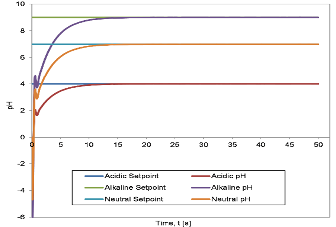
5.1. Servo action
Variable setpoints were provided to assess the controller’s ability to track setpoints. A setpoint of 4 was chosen for acidic control, 7 pH was chosen for neutralization, and a pH value of 9 was chosen for alkaline control.
The corresponding results are depicted in Figures 3 to 5. Figure 3 illustrates the servo response of the system when the controller was tuned using the BFTPSO algorithm. Similarly, Figures 4 and 5 show the servo response of the system when the controller was tuned using the GA and the QFT algorithm, respectively.


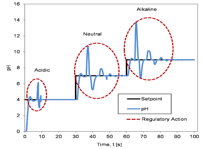
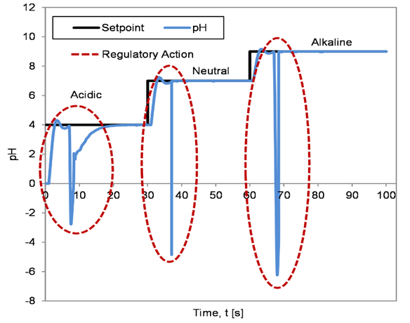
5.2. Servo and regulatory action
The controllers’ ability to track setpoints while also rejecting external input disturbance was tested. Initially, a step input of 4 and a disturbance of +25% of the set value were applied during acidic control. Similarly, a step input of 7 and a disturbance of +14% of the set value were applied during neutralization. Finally, a step input of 9 and a disturbance of +11% of the set value were applied during alkaline control.
The resulting servo and regulatory response of the controllers are depicted in Figures 6 to 8. Figure 6 illustrates the servo and regulatory response of the system when the controller was tuned using the BFTPSO algorithm. Similarly, Figures 7 and 8 show the servo and regulatory response of the system when the controller was tuned using GA and QFT algorithm, respectively.

6. Discussions
The effective controller among the three was deduced by comparing the three controllers’ setpoint tracking capability and servo and regulatory action. In addition, the time domain specifications of the servo response in all three control cases were also compared, as shown in Table 6.
Table 6 Step response characteristics for pH control.
| pH Control | Characteristics | BFTPSO | GA | QFT |
| Neutral | ITAE | 6.09 | 10.86 | - |
| Rise Time | 0.25 | 1.34 | 5.44 | |
| Settling Time | 3.99 | 2.88 | 8.91 | |
| Overshoot | 53.01 | 0 | 0.02 | |
| Undershoot | 6.98 | 2.20 | 66.65 | |
| Alkaline Control | ITAE | 7.84 | 13.55 | - |
| Rise Time | 0.25 | 2.55 | 5.44 | |
| Settling Time | 3.99 | 5.47 | 8.91 | |
| Overshoot | 53.01 | 0 | 0.02 | |
| Undershoot | 6.98 | 17.29 | 66.65 | |
| Acidic Control | ITAE | 3.48 | 2.80 | - |
| Rise Time | 0.25 | 2.55 | 5.44 | |
| Settling Time | 6.12 | 8.60 | 8.91 | |
| Overshoot | 53.01 | 10.95 | 0.02 | |
| Undershoot | 6.98 | 0 | 66.65 |
It can be seen from Figures 3 to 5 and Figures 6 to 8 that all the controllers could track the setpoints and reject the input disturbance quickly.
However, it can be seen from the results stated in Table 6 that, with neutralization, although the BFTPSO controller provided the quickest control action, it generated a response with large overshoots and undershoots. Similarly, the QFT controller generated no overshoots in the response. However, the settling time was more than its counterparts because of slower control action, and it also generated substantial undershoots in the response. Thus, the GA controller was ideal for neutralization as it generated a quick control action with the fastest settling time, with no overshoots and negligible undershoots and error.
The behavior of the controllers for alkaline and acidic pH control was similar, as with neutralization. The BFTPSO controller generated the fastest control action with large overshoots and undershoots. On the other hand, the QFT controller generated the slowest control action with no overshoots and large undershoots in the response. Meanwhile, the GA controller generated a response with significant undershoots in alkaline control and significant overshoots in acidic control. Nonetheless, the GA controller was preferred over the others, as it produced a quick control action with the fastest settling time and lesser overshoots/undershoots.
Thus, the controller tuned using GA produced the desired output response with faster setpoint tracking and fewer overshoots/undershoots for all three types of pH control than the QFT or the BFTPSO algorithm.
7. Real-time implementation
The offline controller gains obtained from the three algorithms, stated in Table 5, were used to implement real-time control of the pH of the reactor tank fluid using NI myRIO-1900 (Figure 9 (a)). NI myRIO-1900 is a reconfigurable input/output embedded device with a Xilinx Zynq-7010 processor comprising a Real-Time (RT) processor and a Field Programmable Gate Array (FPGA) processor for higher resolution, sensitivity and faster response times in real-time applications.

Figure 9 Control of pH neutralization system using NI myRIO-1900 and pH signal conditioning circuit.
In this system, the pH probe and transmitter were calibrated before use, and the output of the pH transmitter ranging from -420 mV to 420 mV was scaled to 0.5 V to 3 V using a signal conditioning circuit comprising IC CA3140, IC TL081, and IC 555 timer, as shown in Figure 9 (b). Then, the output of the signal conditioning circuit was fed as the input to the RIO, and the output of the RIO was used to manipulate the speed of the pump and thereby the flow rate of the alkaline or acid solution to the mixing tank in the system to maintain the pH value, as explained in Figure 10.
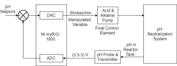
The output of the signal conditioning circuit was fed as the input in any of the referential single-ended or differential-ended analog input channels of the RIO. The corresponding analog output from RIO was converted to 4-20 mA and fed to the pump to manipulate the speed of the pump and thereby the flow rate of the alkaline or acid solution to the mixing tank in the system. Then the control loop was developed in LabVIEW software. The controller configuration and gains were varied in the Front Panel and Block Diagram (Dixit & Jain, 2016). After changing the controller gains, the corresponding results were recorded.
8. Experimental results and discussions
The controller gains in NI myRIO-1900 were varied based on different algorithms like GA, BFTPSO, and QFT, and the accuracy and effectiveness of these algorithms in controlling the pH of the fluid in the reactor tank was found out by analyzing the time domain specifications of the servo capability of the controllers obtained for two test cases of neutralization,
Case 1 - Neutralization of acidic solution (pH = 5)
Case 2 - Neutralization of alkaline solution solution (pH = 8)
In both cases, the neutralized solution had a pH value of 6.5. Figures 11 to 13 depict the servo response of the system when the controller was tuned using BFTPSO, GA, and QFT algorithm, respectively.
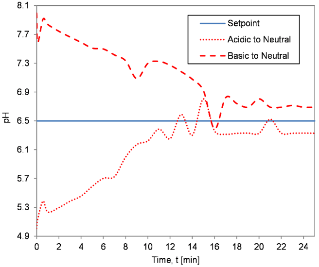


The experimental results indicated in Figures 11 to 13 and Table 7 show that BFTPSO and QFT algorithms generated responses with large settling time. In contrast, GA produced the best response among the three algorithms by generating the desired output response with negligible overshoot, undershoot, and faster setpoint tracking for the neutralization process than QFT or BFTPSO controllers.
Table 7 Step response characteristics for NI myRIO-1900 output response.
| Neutralization | Characteristics | BFTPSO | GA | QFT |
| Acidic To Neutral | Settling Time (minutes) | 22 | 15 | 22 |
| Overshoot | 0.05 | - | - | |
| Undershoot | - | - | - | |
| Offset | 0.17 | 0.18 | 0.18 | |
| Basic to Neutral | Settling Time (minutes) | 21 | 12 | 21 |
| Overshoot | - | - | - | |
| Undershoot | 0.017 | - | - | |
| Offset | 0.19 | 0.18 | 0.13 |
9. Conclusions
In this project, experimental data was acquired from a highly nonlinear multiple input single output pH neutralization system, and linear system models were developed around an equilibrium point. Popular robust and metaheuristic optimization algorithms, like, Quantitative Feedback Theory, Bacterial Foraging Technique based Particle Swarm Optimization Algorithm, and Genetic Algorithm were chosen to deduce the appropriate values of the gain parameters for implementing a PID controller. These controllers were then implemented in real-time to control the pH of the fluid in the neutralization system using a signal conditioning circuit and reconfigurable I/O device. The step response characteristics of the output response from the three algorithms were compared in simulation and experiment, and the genetic algorithm was found to be a suitable algorithm for the real-time control of this system. Furthermore, the genetic algorithm produced output with quicker settling times and negligible overshoot and undershoot, than the QFT or the BFTPSO algorithm.

