1.1. Generic finite elements

The Generic finite elements have been used in problems of finite element adjustment and the identification of parameters. ^{Ahmadian and Jalali (2007)} used generic finite elements to model bolted lap joints. Based on the minimum mathematical requirements, generic stiffness, mass and damping matrices were deduced; the identification of generic parameters was performed looking for the minimization between the Model's Frequency Response Function (FRF) and the measured FRF of a structure that contained an overlap joint. The results were satisfactory, and of particular interest is the fact that the possibility of deducing and employing generic damping matrices was explored. However, the minimum mathematical requirements for damping matrices are unknown and whatever is used, including that presented in ^{Ahmadian and Jalali (2007)}, is not easy to justify.

^{Ratcliffe and Lieven (2000)} proposed a method of identifying general joints based on the use of generic elements and a scheme of minimization of differences in FRF of substructures and FRF of the complete structure. Damping identification was also carried out in this work, although it was not modeled with generic matrices. ^{Titurus et al. (2003)} proposed the use of generic elements for model fit-based damage identification; In their work, the authors show the effectiveness of generic matrices in executing model adjustments when using the inverse sensitivity method. ^{Law et al. (2001)} introduced the concept of Super Element, which consists of formulating hybrid elements composed of several individual elements and three-dimensional models of joints, specified through generic matrices to model stiffness; the effectiveness of the method was evaluated with the adjustment of a three-dimensional truss in the modal domain and it was concluded that the method works to obtain good predictions of low vibration modes. ^{Terrell et al. (2007)} proposed a method for obtaining substructures using generic matrices and constraints for the conservation of model connectivity, and illustrated the fitting process from a trial on an L-shaped structure, using their corner as a substructure.

1.2. Prestress force identification

Prestressing is often employed in civil structures such as bridges, tunnel linings, or other structures requiring long spans while keeping other dimensions comparably small. Prestressed concrete structures constitute effective solutions that optimize the use of materials and provide extended service life (^{Wang et al., 2017}). Nevertheless, the cables and rods that apply the prestress lose tension over time due to steel relaxation and concrete deformations (^{Guo et al., 2018}; ^{Kim et al., 2017}). This loss can cause serviceability problems and the collapse of the structure. Although losses are considered in the design of prestressed elements, the uncertainty associated with diminished tension is significant at any given time during the life of the structure. Therefore, the tension specified in the design is generally not suitable for structural evaluations.

One approach for the identification of prestress forces is the use of dynamic response data from forced vibration tests. The technique uses a finite element model updating scheme that seeks to minimize a normalized difference between calculated and measured dynamic responses. The sensitivity of modal parameters to prestress variations has been studied by ^{Abdel-Jader and Glisic (2019)}, ^{Breccolotti (2018)}, ^{Bruggi et al. (2008)}, ^{Dall'Asta and Dezi (1996)}, ^{Hamed and Frostig (2004}, ²⁰⁰⁶⁾ and ^{Saiidi et al., (1994)}. These studies show conflicting results as to whether natural frequencies increase or decrease with increasing prestressing forces.

Because the effect of prestress on modal parameters in beams is still controversial, some researchers have used time-domain data to identify prestress values. ^{Lu and Law (2007)} formulated the dynamic response sensitivity to parameter changes and illustrated its use via simulations and laboratory tests. ^{Lu and Law (2006)} also presented a methodology to identify prestress forces from time-response data. Their method was based on the formulation of a linear inverse problem that uses the dynamic response sensitivity proposed by ^{Lu and Law (2007)} to construct the rectangular matrix of the model. The method was used to identify the stress in an axial cable in the absence of parameter uncertainty, which was guaranteed in the simulation and the experiment by updating the model before applying to prestress.

^{Lu and Li (2008)} proposed a similar procedure using the Timoshenko beam elements. The effect of the magnitude of the axial force on the effectiveness of the identification was studied, and it was concluded from simulations that the method is not sensitive to the axial force; however, an experimental verification was not provided. In a study ^{by Velez et al. (2010)}, the use of generic finite elements and genetic algorithms to solve the force identification problem was explored. In that case, simulated studies showed that generic elements can be used to account for parametric uncertainty.

Despite the ongoing discussion regarding the effect of prestress on natural frequencies, these have also been used as base data to identify prestress forces. In particular, ^{Kim et al. (2004)} presented a prestress identification method from measurements of 5 natural frequencies whose application is illustrated in a laboratory structure and computational models.

Other authors have focused on predictions and monitoring of prestress losses as a strategy to evaluate the structural safety of prestressed elements^{. Xuan et al. (2009)} considered a pre-stress loss monitoring technique based on fiber optic sensors. The operation of the system was tested in controlled trials and the total losses in different periods were quantified. The authors concluded that the use of this pre-stress loss monitoring technique is viable in operating structures.

Other works on prestress monitoring were developed by ^{Sun et al. (2002)}, where a method for monitoring losses in nuclear containers is presented, and ^{Anderson (2005)}, who showed the results of thirty years of continuous measurement of prestress in a nuclear container.

For all the above, in this paper, a novel and robust method for identifying prestress forces in the presence of modal parameter errors is proposed to remove the limitations presented by the method of ^{Lu and Law (2006)} for the identification of prestressing force. The identification process is posed as an optimization problem that is solved using simulated annealing algorithms. The beams are modeled with generic elements to account for parameter uncertainty, and solutions are sought simultaneously for the parameter of the generic finite elements and the prestress force. The authors described first the methods based on the use of Simulated Annealing and generic finite elements to improve the identification of prestressing force and then presented the effectiveness of the strategy, which was evaluated through numerical simulations and experimental tests on a prestressed concrete beam.

2.1. Simulated Annealing (SA) algorithms

Annealing is a metallurgic process in which a metal is heated to high temperatures, inducing disturbances in the position of its atoms. If the subsequent cooling is sufficiently slow, the metal reaches a stable state and an ordered atomic structure. The numerical simulation of this process is known as Simulated Annealing (SA) and it is employed in Inverse Problems through random alterations of the decision variables (^{Inman et al., 2005}).

A significant number of possible states exist for atoms. Each state, s, has an associated energy E(s); if the system is under thermal equilibrium at a temperature T, the probability of the system being in an s state is defined by the Boltzman distribution

where k is the Boltzman constant and S is the set of possible states. This property is exploited in the following manner in the Metropolis algorithm (^{Levin & Lieven, 1998}): if the system is in the initial state, si, with energy E(si), the alteration of a randomly selected atom will produce a new state sj, with energy E(sj); the new state is accepted or rejected according to the Metropolis criterion: if E(sj) ≤ E(si), the new state is accepted; if the opposite is true, the probability of the new state being accepted is

where although it is possible to improve the performance for axial force is the difference between states of current and former energy and k is the Boltzman constant, which may be taken as unity. The analogy between optimization and thermodynamics is defined as follows: the state of the system is the set of parametric values; energy is the target function; temperature is a control parameter in the process, and the minimum energy is the global minimum. In each iteration, the new state is generated by using a function that specifies new random states with respect to the initial state, and when the possible number of states is depleted, temperature is reduced according to a cooling chronogram (^{Spall, 2003}).

Details of the implementation of Simulated Annealing (SA) algorithms vary significantly depending on the specific problem, and the performance of the algorithm depend on the characteristics or specific values of the initial temperature, the cooling sequence, the transition function, and the stopping criteria. The initial temperature, To, must be selected in such a way that the search is not blocked during the first iterations; if it is too high, too many states will be accepted in each transition and the process will be similar to a random search, and if it is too low, the solution can stall at a local minimum. The current research studied three initial possible temperatures. The cooling sequence characteristic of the Metropolis algorithm contemplates reduction of temperature after the number of available transitions has been depleted or the system has reached a thermal equilibrium. For the purpose of this work, temperature was reduced according to the scheme Ti = αTo, with α = 0.85.

Different alternatives exist to define the transition function. In each iteration, the new state or parameter value can be defined by adding a random increment to one or more parameters at the same time. The new state can also be defined, through random or deterministic selection of a new value for a parameter in each transition, or by adding disturbances according to points on a fixed-radius hyper sphere (^{Spall, 2003}).

In this work, random selection of a vector of parameters in the specific search space was used. Regarding the stopping criteria, the algorithm may be halted according to a specified number of iterations or to some tolerance criterion. The current study employed the freezing criterion, specified here as the temperature at which 90% of the transitions are rejected.

An additional aspect that must be considered in the definition of SA algorithms is the valid range of values for the parameters. In general, as the range broadens, solving the identification problem becomes more difficult. When identifying prestress, it is possible to define reasonable ranges that significantly reduce the search space. For instance, a range can be defined for the axial force according to one of four criteria: i) knowledge of the axial force specified in the design, ii) knowledge of the number and diameter of the strands, iii) estimation of the minimum required stress in the beam according to its dimensions, and iv) estimation of the beam’s elastic critical buckling load. The first alternative may reduce the number of iterations significantly. The second permits estimating the maximum stress that could have been applied to the beam according to the nominal resistance of the strands, which is more or less standard. The third alternative implies the execution of a structural analysis of the element and can provide a good initial approximation at the lower limit. As to the fourth alternative, it may provide a good estimate of the maximum feasible force in the case of slender members. The generic parameters can be restricted according to numerical considerations or to the values known for different types of conventional finite elements. For example, the v1 parameter equals 48 to describe Euler, Timoshenko, and Hughes beams, while for the same beams, the v2 parameter equals 192β, where the constant is a function of geometric parameters and shear effects on stiffness (^{Gladwell & Ahmadian, 1995}). Regarding damping, the range may be specified based on engineering judgment or on experimental data published from measurements on similar structures.

The simulations and the experimental process were executed by combining the criteria of maximum stress on steel and minimum stress required by the system. The SA algorithm implemented in MATLAB@ seeks to minimize the function

In which x¨ and ω denote the acceleration and natural frequency of the beam, respectively and the sub-indices exp and an denote experimental (measured) and analytical (estimated), respectively. Only the frequency from the first vibration mode was included. The system response for each iteration was obtained using the Newmark mean acceleration method for each mode of interest and then calculating the overall response by modal superposition. For the beam model, it was observed that the inclusion of two modes was sufficient to produce accurate results. For simulations, as well as for the experimental procedure, the search space restraint approach was employed. Hence, the minimum required force was taken to be the force required for the beam to withstand its own weight, and that the initial prestressing force was assumed to be known. For the experimental procedure, the assumption was made that the axial force had a loss of 20%, which is a reasonable approximation of the initial losses in a prestressed beam. Additionally, the v1 generic parameter was taken to be a constant value of 48, as in several types of known beams, v1 is defined with this value, so that it may be left fixed and damping can be included in the identification problem without increasing the number of parameters. A similar reasoning was employed by ^{Ahmadian and Jalali (2007)} to identify joints.

2.2. Generic finite elements

Generic finite elements were formulated by ^{Gladwell and Ahmadian (1995)}. The authors demonstrated that the mass and stiffness matrices obtained with the finite element method, for different types of elements, belong to a family of elements that can be represented by a single matrix. Generic element matrices can be deduced from any of the family members; that is, the mass and stiffness matrices of the Euler-Bernoulli beam can be used, for example, to deduce the stiffness matrix of the generic beam, of which the Euler beams, Timoshenko, among others, are particular cases. The use of this type of element is particularly useful in inverse problems since the matrices are represented uniquely by few parameters, as long as the traditional physical parameters are defined with sufficient precision. After the formulation of generic finite elements, it was used in problems of finite element adjustment and identification of parameters.

Generic finite elements are formulated from the following general characteristics of the mass and rigidity matrices (^{Gladwell & Ahmadian, 1995}):

Given that the prior characteristics are the only mathematical requirements for an element’s mass and stiffness matrices, these can be used to specify families of elements that fulfill these basic requirements.

The free vibration of an element is governed by the Equation

Where

The geometric stiffness matrix is written for the i^th element of a beam as

The Ti factor is the axial force applied to the ith element. In the present context, it represents the prestressing force.

By modifying the eigenvalues λ and eigenvectors Φ from the eigenvalue problem (Eq. 4) in such a way that the basic requirements for mass and stiffness matrices are fulfilled, the generic finite element matrix for a beam is obtained as (^{Gladwell & Ahmadian, 1995}).

where ko = EI/L. Thus, E, I, and L parameters may be omitted in the solution of Inverse Problems, so that the beam depends only on two parameters, v1 and v2. As mentioned in Section 2.1, ^{Gladwell and Ahmadian (1995)} showed that the various classical beam models are special cases of the generic beam. For instance, v1 = 48 to yields Euler, Timoshenko, and Hughes beams. For these beam types v2= 192β₁, where the constant β₁ is a function of geometric parameters and shear effects on stiffness. When generic beams are employed, the degrees of freedom of the element are

and, consequently, the responses associated to the degrees of freedom 2 and 4 of the element must be divided by the length of the element to obtain rotation units.

2.3. Experimental setup

Fig 1 shows the setup used in the experimental study. The simply supported beam has dimensions (bxhxL) of 25 x 30 x 395 cm, with a 5/8-inch tendon placed concentrically, without grouting, in a 1-inch duct. The beam was post-tensioned to 196,133 N force using a hydraulic jack. The applied force was measured with a load cell installed between one of the anchorages and a steel plate provided to reduce stress concentrations (Fig 2). After removing the jack, the cell registered a value of 153,964.41 N.

Figure 1 Experimental Setup. 

Figure 2 Detail of the load installation. 

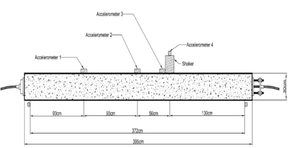
To obtain the initial modal properties of the system, a modal test was performed to measure the Frequency Response Function (FRF) of the beam and calculate the fundamental natural frequency and the modal damping associated to the first vibration mode. An initial sinusoidal sweep was carried out between 0 and 100 Hz at a rapid rate to find a fundamental resonant frequency. This was observed around 27 Hz and its identification was refined by consequently conducting a slower sweep between 26 and 29 Hz. Through an analysis of the FRF it was established that the fundamental natural frequency was 27.68 Hz. The analysis was performed through the circle fit method (^{Ewins, 2002}). According to the analysis, the equivalent viscous damping ratio of the first mode is 3.24%. The axial force was then reduced in a controlled way by gradually displacing a threaded mechanism that was installed between the beam and the tendon anchorage on the end opposite to that of the load cell (Fig 3). A minimum value of 118, 268.20 N, according to the load cell reading, was achieved. The modal analysis process was repeated for a total of five different axial force values and insignificant variations in the natural frequency and the damping ratio were obtained.

Figure 3 Detail of the guide for the variation of the prestress force. 

3.1. Simulated Annealing (SA) algorithms

The simulated structure is a simply supported, 20-m long beam, with a 25 cm x 30 cm cross-section, 3% damping for all modes, modeled with Euler-Bernoulli elements. The excitation is a sinusoidal force whose frequency is close to the beam’s first natural frequency. The beam’s mass and stiffness matrices were first assembled and used to calculate the first natural frequency using MATLAB’s built-in function for eigenvalues. The resulting natural frequency varies slightly depending on the prestress force. Therefore, excitation frequency was set at an arbitrary value of 28 Hz, and the resulting dynamic force applied to the simulated beam was P = 400 sin [2π(28)t] N.

The response was obtained using the Newmark mean acceleration method for each mode of interest and then calculating the overall response by modal superposition (^{Chopra, 1995}). The reference response for the simulations is vertical acceleration at 3 m from the left support. Since the simulated beam is an Euler-Bernoulli beam, its stiffness matrix is equivalent to having v1 = 48 and v2 = 192.

The “model” is the beam itself but modeled with generic elements. For this beam, v1 is fixed at 48, and the identification procedure is carried out to calculate v2, the axial force, and the modal damping for the first mode.

Table 1 shows the results of the simulations for three different forces in which an initial temperature of 50,000 was specified, along with 300 transitions, and 1,000 energy levels. It can be seen that as the force increases the identification of the parameters improves; this can be explained from the stiffness matrix expressed in Eq. 5, in which it is evident that the stiffness degrades as the force increases and therefore, the greater the pre-stress, the beam will be more flexible.

Although the results of the simulation are promising, it must be understood that the associated computational cost is high and, therefore, it is justifiable to look for an alternative to achieve a faster solution. Consequently, the use of Adaptive Domain Restrictions is proposed to accelerate the convergence of the process. The strategy is to modify the lower limit of the search space each time the energy is reduced. The new lower limit is calculated from the state that produced energy reduction as

where vector R is a vector operator and the symbol "*" denotes one-to-one multiplication. The operator may be diverse; It can be an algebraic, binary, differential operator, among others. The question of what the form and content of the operator should be according to the specific problem is left open. In this work, however, an algebraic operator whose elements are equal to unity is used. Table 2 shows the simulation results to identify a force of 200,000 N. Except for the fourth experiment, all the results are between 1% and 10% of error, which shows the potential that the strategy has to improve the results while reducing the computational cost, since only 2 levels of Energy were used. However, it is required to investigate which operators can guarantee that the adaptive constraints do not produce solutions that imply an overestimation of the axial force.

3.2. Experimental identification of the prestress force

Prior to identification, the initial finite element model was adjusted to minimize the initial error. Careful definition was exercised for the physical and geometric parameters, as well as for the finite element mesh size, and the following values were used: E = 24.5 x 10^⁹ N/m², ρ = 2,400 kg/m³, and a 20- element mesh. The stiffness matrix was defined according to Eq. 5 and the mass was modeled with consistent matrices (derived from shape functions). The axial force was introduced by using the geometric stiffness matrix (Eq. 6).

Identification was performed by using the same scheme as used for the numerical simulations, i.e., seeking minimizing values for the v2 generic parameter, the axial force, and the equivalent viscous damping ratio, and specifying domain constraints. The search was conducted over the range of 80,000-180,000 N for the axial force, 2-192 for v2, and 0.01-0.05 for the damping ratio. The excitation used corresponded to the first two seconds of the sweeps used for identification. Three different initial temperature levels were evaluated to avoid solutions blocked at high temperatures or low temperatures. How was mention below it was assumed that the axial force had a loss of 20%, which is a reasonable approximation of the initial losses in a pre-stressed beam. Additionally, the v1 generic parameter was taken to be a constant value of 48, so that it may be left fixed and damping can be included in the identification problem without increasing the number of parameters. Tables 3 to 5 show the results of five identification runs for the 153,964.41 N force at temperatures of 5,000, 50,000, and 100,000. According to the results, the temperature at 50,000 presents lower dispersion and, hence, its results are considered most suitable to make decisions and draw conclusions.

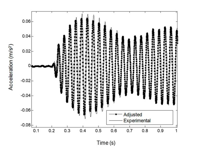
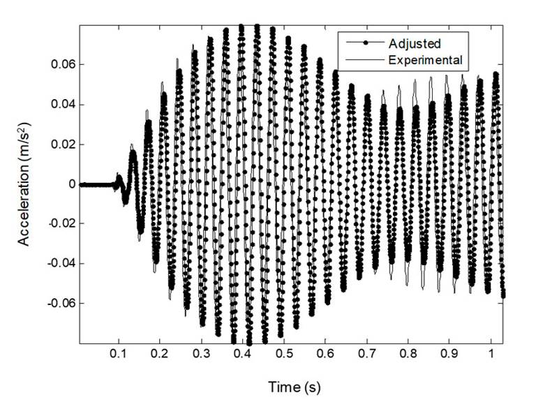
The 153,964.41 N axial force was identified with a 4.47% maximum error and a 1% minimum error (Tables 3 to 5). It is worth mentioning that the minimum error was an overestimation of the force, therefore this result should not be considered adequate from the point of view of structural safety. Nevertheless, the results are encouraging and show the potential effectiveness of the method. Fig 4 and Fig 5 show that the calculated responses after the identification process (dotted line) correspond adequately with the experimental results (continuous line).

Figure 4 Experimental response and adjusted response - P = 153,964.41 N. 

Figure 5 Experimental response and adjusted response - P = 118,268.20 N. 

Damping was calculated with a 34.8% maximum error and a 1.7% minimum error. In this case, data dispersion was significant, as shown in Table 2. It is considered that damping was not successfully identified. Also, the v2 generic parameter shows a clear tendency to being well below the upper theoretical limit. This result can be physically interpreted as an indicator of the effect of the shear force on the stiffness of the beam. If v2 is defined as:

where

and C is a shape factor, the Timoshenko beam is obtained. In this case, the constant C can be interpreted as the effect of the reduced stiffness (see Discussion below). This shows how generic elements allow a greater degree of approximation in the inverse problem. Regardless of the interpretation given in terms of the type of element identified, the point is that reduced stiffness was observed, which would have been difficult to discern without recurring to arbitrary modifications of the physical parameters if the beam had been modeled with Euler-Bernoulli elements or another classic formulation. In other words, a model that produced a satisfactory fit was obtained, with physical, geometric, and kinematic parameters that have a reasonable physical interpretation, regardless of the value of the generic parameters.

Tables 6 to 8 show the results of the identification of the 118,268.20 N force. Again, the temperature at 50,000 produced results with lower dispersion. The identification results show that although greater difficulty was encountered in detecting the axial force, the values identified seem to be slightly greater or less than the desired value. Therefore, it can be assumed that with a greater number of experiments, the force could be approximated with a statistical treatment of the results from each experiment. ^{Lu and Liu (2008)} observed a similar phenomenon for low axial forces.

3.3. Discussion

The simulation results provide several interesting observations. It is evident that a greater axial force yields better identification results. This is true for the model of Eq. 5, which in essence is a stability model in terms of stiffness. According to this model, an axial force limit exists that would completely nullify the stiffness, that is, a buckling critical load. However, experimental data reported in the literature and observed in the present research appear to show that an increase in the prestress force causes an increase in stiffness. It is clear that a gap in knowledge exists in this sense. From the perspective of static behavior, it is hard to argue with the fact that stiffness is reduced by second-order effects induced by an axial force, yet experimental evidence shows a tendency to the contrary. A possible explanation is that in practice the tendon comes into contact with the duct walls during motion and this causes an increase in the effective rigidity (^{Dall'Asta & Dezi, 1996}). This increased stiffness may also affect the identified generic values by tilting the results toward a stiffer behavior. This stiffening effect is plausible in the beam studied in the current work and in similar beams studied elsewhere because the ducts had diameters that were only slightly greater than those of the strands, which makes contact more likely.

The Adaptive Constraints approach is a heuristic strategy that promises to improve the speed of SA algorithms. However, instructions that involve too many calculations should not be included to specify the R operator, as computational savings could be compromised. In this work, the binary operator without zeros was used, whose effect is simply to replace the initial lower limit with the new state in each transition that produces energy reduction. Although the axial force showed a tendency to overestimate with this approach, the results were more satisfactory in terms of computational cost and identification of generic parameters, although it is possible to improve the performance for axial force if its upper limit is known with precision.

The fitting variables in the problem are continuous, and as discussed previously, in an application in which prestress needs to be identified with the method described above or with any other method that involves optimization, the analyst can specify constraints with physical justification. In fact, the linear methods presented in ^{Lu and Law (2007)} and ^{Lu and Liu (2008)} have an implicit constraint: the initial error must be small. In the opinion of the authors, these linear schemes cannot be effective if the initial errors are large, let alone when uncertainty exists in parameters different from the axial force.

The values calculated for the generic parameter v2, are well below the values that correspond to the known beam models. However, the fact that it is below the value for Euler's beams - which seems to be the upper limit in the family of elements of four degrees of freedom - is consistent with what would be expected from a beam with the dimensions of the studied beam, that is, it behaves more like a shear beam. Besides, the purpose of the generic elements was fulfilled: that an adjustment of models is achieved respecting the logical values and with a clear sense of the parameters of the material, the cross-section, and the kinematic restrictions (supports). As for the damping, it cannot be stated that it was identified, but at least the values found in the different simulations were reasonable.