


 text new page (beta)
 English (pdf)
 Article in xml format
 Article references
 Send this article by e-mail
 Cited by SciELO
  Similars in
SciELO
Similars in
SciELO 
 Permalink
1. Introduction
Today’s business organizations are working in an environment where there are threats from everywhere such as it competitors, uncertain market conditions and so on. Haghighat et al. (2013) studied the predictive models future can be forecasted with a certain degree of accuracy by exploiting the patterns obtained in historical data and transactions. Building a Predictive Analytics model helps to assess risks using a certain set of conditions and helps organizations to improve their business.
Nelder (1978) explored the Predictive Analytics focuses on getting the events of the future by analyzing the past data. Svetnik et al. (2003) discuss the classification and regression techniques play a major role in machine learning and data mining applications. Using these techniques, future can be predicted. In a supervised learning model, the algorithm learns on a labeled dataset, providing an answer key that the algorithm can use to evaluate its accuracy on training data by Quinlan (1986).
Keerthi & Gilbert (2002) focused on the unsupervised model, which provides unlabeled data that the algorithm tries to make sense of by extracting features and patterns on its own.
The proposed model makes use of logistic regression to predict whether a customer can purchase a sport-utility vehicle or not by analyzing the various fields such as User ID, gender, age, and estimated salary of a customer.
The rest of the paper is as follows. In Section 2, we discuss about Literature Survey. In Section 3 we discuss the basic concepts of logistic regression. In Section 4 we discuss the data cleaning, data wrangling, filling the missing data and framing the data model. In Section 5, classification report is given. In Sections 6 and 7, the confusion matrix and the accuracy score are obtained. Finally, Section 8 describes the conclusion and future work.
2. Literature survey
Uyanik and Güler (2013) described the statistical technique for estimating the relationship among variables which have reason and result relation. They analyzed the student’s performance in their University. Zekic-Susac et al. (2016) explained the company's growth by applying the logistic regression and neural network technique. They tested the model without variable reduction. They got more accuracy while applying neural network technique. The accuracy of the model was compared using statistical tests and ROC curves. Peng et al. (2002) stated that the application of logistic methods with an illustration of logistic regression. They applied to a dataset in testing research hypothesis. Pyke and Sheridan (1993) analyzed 477 masters and 124 doctoral candidates at a large Canadian university. They considered various parameters like demographics, academic and financial support variables to analyze the dataset. They found out whether a student completed the degree or not.
3. Introduction to regression models
A. Logistic regression:
Logistic regression is a predictive modeling analysis technique. It is used in the machine learning for binary classification problems. The logistic regression algorithm defines the statistical way of modeling and the outcome is binomial. The outcome should be discrete or categorical variable such as Pass or Fail, 0 or 1, Yes or No, True or False, High or Low. The dependent variable in logistic regression is binary. Dependent variable is also referred to as "Target variables". Independent variables are called the "Predictor variables".
Logistic Regression predicts the probability of the event using the log function. The sigmoid function/curve is used to predict the categorical value. The threshold value decides the outcome (win/lose).
Linear regression equation:
y holds the dependent variable that needs to be predicted.
ß0 is Y-intercept (Point on the line that touches the y-axis).
ß1 is the slope (The slope can be negative or positive depending on the relationship between the dependent variable and the independent variable.)
X here denotes the independent variable that is used to predict our resultant dependent value.
Sigmoid Function:
Apply sigmoid function on the linear regression equation:
Sigmoid function is also called as logistic function and gives output as s curve that lies between the value 0 and 1. If the s curve goes to positive infinity, then the predicted y becomes 1 and if the s curve goes to negative infinity then the predicted y becomes 0.
In this research “y” refers to purchased column and “X” refers to age and estimated salary columns.
When the number of possible outcomes is only two, it is called binary logistic regression.
In this research, binary logistic regression is used and the prediction confirms whether the customer can purchase the sport-utility vehicle or not.
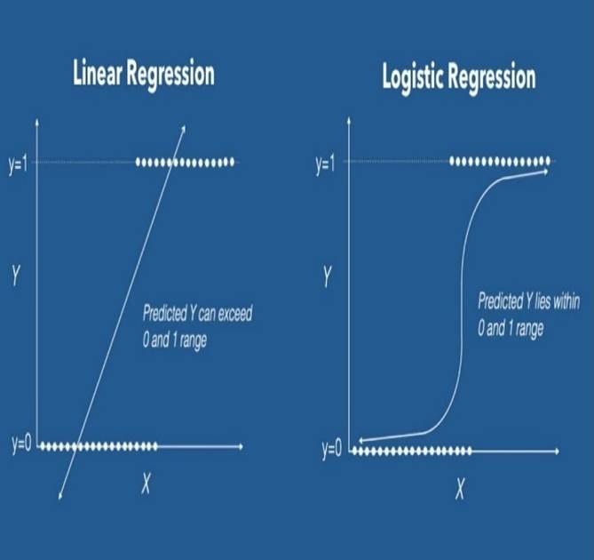
B. Linear vs. logistic regression:
Linear regression can have infinite possible values. Logistic regression has definite outcomes.
Linear regression is used when the response variable is continuous in nature, but logistic regression is used when the response variable is categorical in nature.
The output of linear regression is straight line, whereas the output of the logistic regression is s-curve as shown in Fig.1.
C. Proposed work:
In this proposed work, totally 1001 records have been taken for a dataset as a CSV file. In Exploratory Data Analysis (EDA), data wrangling, missing data, data cleaning and converting categorical values are done by using python library and built-in functions. After splitting the dataset into training and testing data, the model is fit using logistic regression using scikit learn library. After that classification report is obtained. At last confusion matrix is found to calculate the accuracy score of the model. The following sections explain it in detail.
4. Data analysis and prediction
Figure 2 shows, how the model is implemented. The following steps are carried out to produce the result.

Collecting data:
The very first step for implementing the logistic regression is to collect the data. The CSV file containing the dataset is loaded into the programs using the pandas.
Importing libraries and dataset:
Cherian et al. (2008) experimented the Panda’s library is used for data analysis; Matplotlib library is used for data visualization; NumPy is used for numerical analysis and array manipulations.
Seaborn library is a Python data visualization library based on Matplotlib. It provides a high level interface for drawing attractive and informative statistical graphics.
While using Jupyter Notebook, %matplotlib inline is written for displaying the plots in the notebook.
In this work, aliases are used for the imported libraries such as ‘pd’ for Pandas, ‘plt’ for Matplotlib, ‘sns’ for Seaborn, ‘np’ for NumPy, ‘sklearn’ for SciKit learn machine learning models. This has been done for our convenience so that these libraries and the methods can be invoked with these aliases instead of writing the full name of the library.
Data Set:
The training data set is now supplied to machine learning model, on the basis of this data set that is trained. The classification goal is to predict whether the customer will purchase (1 / 0) SUV or not. The dataset provides the SUV sales customers’ information. It includes 1001 rows and 5 columns. Table 1 describes the structure of the dataset. Table 2 shows the first 5 records of the dataset. Table 3 shows the last 5 records of the dataset.
Table 1 Structure of the dataset.
| Variable Name | Description | Type |
| User ID | Unique User ID | Integer |
| Gender | Male / Female | String |
| Age | Age in numbers | Integer |
| Estimated Salary | Salary in thousands | Double |
| Purchased | Car Purchased (1 / 0) | Integer |
Table 2 Head records of the data set
| User ID | Gender | Age | Estimated Salary | Purchased | |
|---|---|---|---|---|---|
| 0 | 15624510 | Male | 19.0 | 19000.0 | 0 |
| 1 | 15810944 | Male | 35.0 | 20000.0 | 0 |
| 2 | 15668475 | Female | 26.0 | 43000.0 | 0 |
| 3 | 15603246 | Female | 27.0 | 57000.0 | 0 |
| 4 | 15804002 | Male | 19.0 | 76000.0 | 0 |
Table 3 Tail records of the data set.
| User ID | Gender | Age | Estimated Salary | Purchased | |
|---|---|---|---|---|---|
| 996 | 85691863 | Female | 46.0 | 41000.0 | 1 |
| 997 | 85706071 | Male | 51.0 | 23000.0 | 1 |
| 998 | 85654296 | Female | 50.0 | 20000.0 | 1 |
| 999 | 85755018 | Male | 36.0 | 33000.0 | 0 |
| 1000 | 85594041 | Female | 49.0 | 36000.0 | 1 |
Analyzing data:
The dataset is analyzed using the variables by creating different plots to check the relationship between the variables.
Figure 3 Number of customers who have purchased an SUV or not.
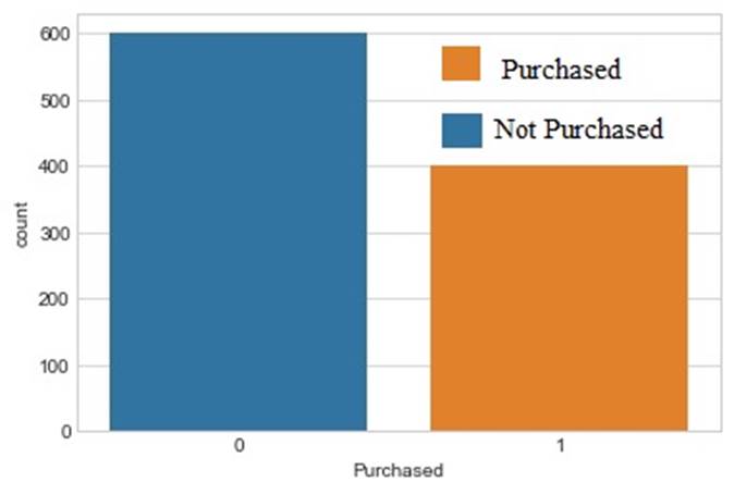
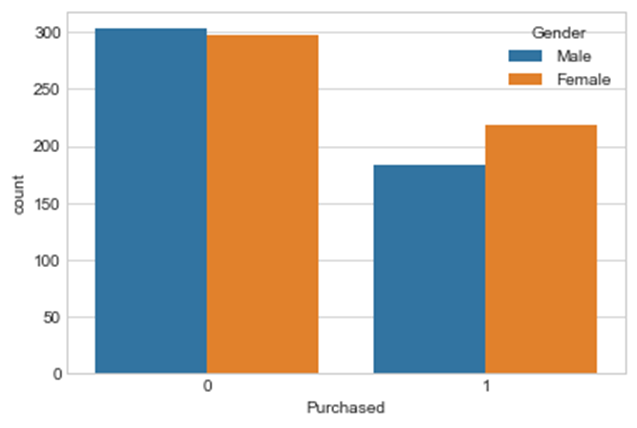
Figure 4 shows the number of customers who have purchased SUV or not across gender.
Exploratory data analysis:
Exploratory Data Analysis (EDA) is the first step in the data analysis process.
Data wrangling:
Data Wrangling means cleaning the data by removing the NAN (Not a Number) values and unnecessary columns in the dataset which are modified according to the target variable. All the null values and the string values will be eliminated from the Data Frame.
Missing data:
Seaborn library can be used to create a simple heatmap to see where the data is missed.
sns.heatmap(data.isnull(),yticklabels=False,cbar=False,cmap=’viridis’)
Figure 5 shows the dataset consisting of NAN values.
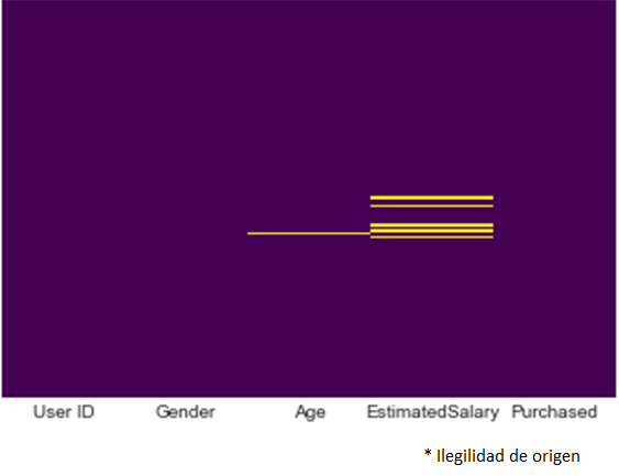
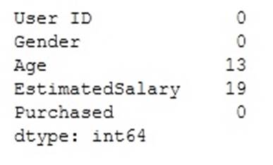
Figure 6 describes the total NAN values for age which is 13. Similarly, for the estimated salary which is 19.
All the irrelevant data will be checked (null values) and the values need not be required while building the prediction model. If there are no null values in the sales dataset, it will be proceeded with splitting the data.
Data cleaning:
To replace the NAN fields, the “Mean” value will be filled instead of just dropping the missing data rows.
data [‘Age’].fillna(data[‘Age’].mean(),inplace=True)
Table 4 describes the count, mean value, standard deviation value, minimum value and maximum value for age, estimated salary and purchased columns.
Table 4 Output of describe () table
| User ID | Age | Estimated Salary | Purchased | |
| count | 1.001000e+03 | 988.000000 | 982.000000 | 1001.000000 |
| mean | 4.117609 e+07 | 38.978745 | 69303.462322 | 0.400599 |
| std | 2.623339 e+07 | 10.743418 | 34320.869568 | 0.490265 |
| min | 1.556669e+07 | 18.000000 | 15000.000000 | 0.000000 |
| 25% | 1.572337 e+07 | 32.000000 | 42250.000000 | 0.000000 |
| 50% | 3.557437 e+07 | 38.000000 | 65000.000000 | 0.000000 |
| 75% | 6.568749 e+07 | 47.000000 | 88000.000000 | 1.000000 |
| max | 8.581455 e+07 | 77.000000 | 150000.000000 | 1.000000 |
Converting categorical features:
Categorical features have to be converted into dummy variables using Pandas. Otherwise, machine learning algorithm cannot be fed with the features as input.
Gender_Status=pd.get_dummies(data[‘Gender’],drop_first=True)
Train and test data:
For the performance of the model, the data is split into the test data and train data using train_test_split. The data split ratio is 70:30.
As a model prediction, the logistic regression function is implemented by importing the logistic regression model in the sklearn module.
The model is then fit on the train set using the “Fit” function. After this, the prediction is performed using the “Prediction” function.
Figure 7. Output of predicting test results that consist of 1 means customer who have purchased and 0 means customer who have not purchased a sport utility vehicle.

5. Classification report
The classification report displays the Precision, Recall, F1 and Support scores for the model as shown in Figure.8.
Precision is calculated as the number of correct positive predictions divided by the total number of positive predictions.
Precision= True Positive / True Positive + False Positive
Recall is calculated as the number of correct positive predictions divided by the total number of positives. Recall is also known as Sensitivity.
Recall = True Positive / True Positive + False Negative
F1 and Support scores are the amount of data tested for the predictions.
F1 score is the harmonic mean of Precision and Recall.
F1 = 2 x (Precision x Recall / Precision + Recall)

6. Confusion matrix
Confusion matrix is shown in Table 5 that describes the performance of a prediction model. A confusion matrix contains the actual values and the predicted values. These values can be used to calculate the accuracy score of the model.
The four outcomes are formulated in 2*2 matrix, as represented below,

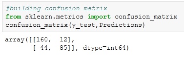
Figure 9. Total value of true negative and positive that are 160 and 85. Similarly, false negative and positive; which are 44 and 12.
7. Accuracy score
Accuracy is calculated as the number of overall correct predictions divided by the total number of the dataset.
81.39 % of accuracy score is obtained by using this logistic regression model for 70:30 split ratio as mentioned in Table 6.
8. Conclusion
The data set have been tested in 3 different split ratios like 70:30, 75:25 and 80:20. 81.39% of customers are interested in purchasing sport-utility vehicle for the train-test split ratio of 70:30; 83.67% of customers are interested in purchasing sport-utility vehicle for the train-test split ratio of 75:25 and 73.13% of customers are interested in purchasing sport-utility vehicle for the train-test split ratio of 80:20. Using this Binary Logistic model, it can be predicted that whether a customer can purchase a sport-utility vehicle or not.
In future, this model can be applied to an enhanced cloud platform with larger volume of data keeping the algorithm remains the same using machine learning deployment for predicting the customer mindset in purchasing a sport-utility vehicle.

