


 nova página do texto(beta)
 Inglês (pdf)
 Artigo em XML
 Referências do artigo
 Enviar este artigo por email
 Citado por SciELO
  Similares em
SciELO
Similares em
SciELO 
 Permalink
1. Introduction
High power lasers in manufacturing are used for cutting, welding, marking, drilling, surface treatments and powder processing on a variety of materials ranging from metals, to polymers and natural materials like leather or stone. Low power lasers are increasingly applied for optical inspection, by measuring position, distance, speed and surface properties like roughness and gloss.
The optimal selection for a given application of a laser source and its processing parameters, namely spot size and energy distribution, requires the characterization of the laser beam geometry and quality.
This paper introduces the most relevant laser beam parameters in manufacturing and describes the development of an apparatus to optically control the laser beam and measure these parameters by image analysis.
International Organization for Standardization (2005) methods and standards for the laser beam characterization have been described in the literature (López & Villagómez, 2015) and are commercially available. The beam quality can be measured by a Shack-Hartmann wavefront sensor. Among the most consolidated are Yan et al. (2018), Sheldakova et al. (2007) and Schäfer et al. (2006). More sophisticated (and complex) methods have no moving components (Schulze et al., 2015), are based on entropy (Porras et al., 2017) or optical resonation (Kwee et al., 2007). A general review of commercial instruments used in beam analysis is available in Roundy (2000), however several technical aspects to achieve a fully functional setup are not available; in particular a camera sensor model is proposed to design the noise filter. Some works describe methods for the analysis of the beam profile with camera sensors. A CCD camera is used in Schweinsberg & Van Woerkom (1999) to characterize the M 2 of a Ti-Sapphire laser; a movable lens permits the modification of the beam section scanned by the camera. Another lens provides the spot magnification, imposing a long distance between lens and camera. A method to estimate the deviation of the beam from an ideal envelope is presented in Denisov & Karasik (2009). A general principle for layout design of a camera-based laser analyzer is described in Alsultanny (2006). Educational experiments with low cost setup, including the characterization of a Gaussian beam, are described in Andrews et al. (2007).
This work starts from recalling mathematically and physically the laser quality, namely beam waist, divergence, Rayleigh range and M 2, which have greatest interest in industrial applications. This article focuses on the design and development of a simple and low-cost laboratory apparatus to optically control the laser beam and measure these parameters by image analysis. Possible measuring strategies are critically compared, sensor design is discussed and experimental validation is provided.
2. Laser beam parameters
2.1. Gaussian beam model and quality parameters
Laser beams are spatial and time high coherent electromagnetic waves presenting a preferred direction of propagation.
The fundamental model for a laser beam is the Gaussian beam with TEM00 intensity distribution shown in Figure 1(a). This simplest case can be described by an axial-symmetric model with just two (polar) coordinates.

Figure 1 Intensity distribution of a Gaussian beam (a) and lower order modes (b, c). Intensity distribution of a real mixed mode and/or optically distorted beam (d).
The propagation and the transverse axes z and ρ are represented in Figure 2. The intensity function I(ρ,z) (Figure 2, detail) is the time-averaged power density with Gaussian shape:

The beam radius w(z) is the conventional beam width on the ρ axis and is expressed as
Where
This function is defined by three parameters that characterize the Gaussian beam summarized in Table 1.
Table 1 Laser parameters for a Gaussian beam.
| Parameter | Symbol | Description |
| Beam Waist |
|
W 0 represents the smallest radius reached by the beam along its path |
| Divergence (half-)Angle |
|
The region in which |
| Rayleigh Range |
|
At a distance equal to zR from the beam waist, the beam radius is |
These parameters affect the laser beam quality and can be estimated by the apparatus described in this paper and are synthesized by the standard Beam Quality parameter M2 defined below.
2.2. Beam quality
The most common parameter to quantify the beam quality is the M 2 parameter. It can be used to characterize also lower order laser beams, with the intensity distribution shown respectively in Figure 1(b, c and d). As described in Siegman (1997), in a resumption of the previous work in Siegman (1993), M2 is related" and keep going with to the focusing capability of the laser on a narrow spot at a given divergence angle. The best possible beam quality (lower M2) is achieved for a diffraction-limited Gaussian beam, which is a particular solution of the paraxial approximation of the equation wave in (1) and (2) having M2 = 1 (M2 minimum). Many real lasers approach this value, especially low power single mode lasers. High power lasers can have a very large M2 of more than 100 or even well above 1000.
Better beams (lower M2) have the following benefits: they allow locating the laser source farther from the working surface, preventing damages to the laser source due to heat and material ejection (Figure 3, top); in laser delivery systems (like optic fibers) higher quality beams propagate at narrower beam size; hence smaller and cheaper optics can be used (Figure 3, bottom); beams remain collimated for a longer distance, increasing the tolerance for longitudinal alignment.

2.3. Real Beams and M 2 Parameter
The beam quality M 2 parameter adapts the Gaussian model to a real beam. It quantifies the quality in relation to the similarities between a real beam and a Gaussian beam. For real lasers two parameters are necessary: M 2 x and M 2 y . M 2 x is defined as:
where W(0,x) and θ(r,x) are the beam waist and the divergence angle of the real beam with respect to the x axis, after focalization; BPPreal and BPPGaussian are the Beam Product Parameters of the examined laser and the ideal Gaussian beam. Similar expressions can be derived for the y axis. An extended discussion is available in Paschotta (2011) and Alda (2013).
The lower case w is used for the Gaussian beam model; the upper case W is used for parameters obtained from operation of the apparatus and from simulations.
It can be noticed that M 2 represents the ratio between the beam waist radius of the real beam and the beam waist radius of a Gaussian beam with the same divergence angle. M 2 defines the shape of the real beam along the z-axis, in that it defines the specific curve of the family in (2) In addition, it includes the information on ( and on the product W0 θr, which are known and constant for a given laser.
Most real lasers are not Gaussian and require a different formulation for the beam radius W(z) by means of second moments, as detailed below.
2.4. Second moment definition of the beam radius
The parameters W 0 and M 2 completely define the beam propagation. When the beam is not axial-symmetric, as for most real lasers, the beam radius can be defined by the second moment of I(x,y), where the ( axis is substituted by the principal axes x and y as in Figure 1(d). The radius propagation function in (1) and (2) become:
Where:
which are used by the image analysis software developed for the apparatus. Similar expressions can be derived for the y axis.
2.5. Characterization methods
The beam parameters M 2 x , M 2 y , W 0,x and W 0,y in (4) are calculated from the measures of the beam radius W(z) at several positions (e.g., 10 positions, with current setup) along the beam path. To estimate the beam waist W 0 and to calculate M 2 two methods are available from ISO (2005) and Siegman (1997). The algorithms based on these methods have both been implemented for redundancy and are outlined for comparison in Table 2.
Table 2 M2 estimation strategies.
| Divergence Procedure (ISO, 2005): |
|
|
| Second Moment Procedure (Siegman et al., 1997): |
|
|
The first algorithm requires the separate estimation of the beam waist W0,x and of the divergence angle θr,x. The second algorithm permits to evaluate the parameters by fitting from images distributed in a shorter part of the beam path.
3. System design
The measurement of the M 2 parameter requires the acquisition of images of the beam sections along the beam path. This task is accomplished reshaping the laser beam using an optical hardware and by collecting a series of images by means of a computer-controlled camera.
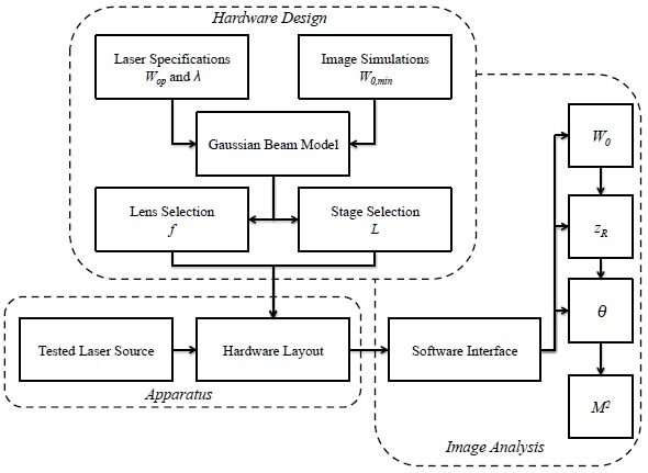
Figure 4 outlines the strategy for the development of the apparatus, which includes two modules described in detail below, the optical system (hardware) and the image analysis algorithm:
the hardware layout reshapes the beam to take measures both in the far and near field;
the software interface controls the image acquisition and analysis to characterize the laser beam.
The laser beam intensity distribution is measured by a CMOS sensor. A CCD has not been selected for the higher cost.
Figure 5 shows a prism mounted on a rail guide. The linear displacement of the prism varies the laser section being acquired by the camera. The beam reflection by the prism permits to use a shorter rail guide, saving space on the platform, as opposed to facing the camera directly towards the laser source. Moreover, it reduces the apparatus size also in the transverse direction as opposed to a couple of mirrors. It also allows keeping the camera fixed, avoiding the movement of this cabled device.

Figure 5 Scheme of the hardware layout. The camera records the beam intensity. The movement of the prism permits the collection of images along the beam path.
3.1. Design of the optical system
Among the main hardware modules, in addition to the rail guide and the digital camera, is the focusing lens (Figure 5). Commercial lasers are usually equipped with an internal optical system to minimize divergence and technical specifications include a nominal exit beam radius W op in addition to the wavelength (.
As shown in Figure 4, to design the apparatus, the focal length f and rail guide length L are selected based on these latter parameters and simulations of the Gaussian beam model, described below.
The main purpose of the lens is to reshape the beam as in Figure 2.The focal length should satisfy the following trade-off:
minimizing the Rayleigh range, influencing the rail guide length L and
keeping the beam waist above a minimum measurable size (approximately 10 pixels) which depends on the camera sensor resolution.
The camera resolution is critical for this aim. A simple camera model derived from those discussed in Lanzetta & Culpepper (2010) has been implemented to simulate the effect on the estimation of the beam radius caused by the spatial discretization and the intensity level quantization. These simulations provide a lower limit for the beam waist, which is used for the lens selection
4. Simulated image analysis
The main input for the apparatus design is the smallest measurable beam radius and it has been estimated by computer simulations according to the following model.
To simulate the image acquisition, each pixel p ij is treated like an integrator of the light intensity generated by the laser
for all the rows and columns of the simulated image p(i,j), 1≤ i≤ N, 1≤ j ≤ M. The intensity from (1) has been simulated for a set of 10 radii W (x,sim)=(1,2,..,10) pixels (Figure 6). p ij is proportional to the energy collected during the exposure time T, on the area A ij of the incident pixel.

The simulated intensity p
ij is then quantized to set the output range between 0 and 255, simulating the compensation in the exposure time to avoid image saturation. Finally, random noise
The conventional radius along the principal axis x estimated from simulated images in discrete form, derived from (5) and (6) is:
where i0 is the x coordinate of the centroid of image p255 (i,j) and is calculated as x0 from expression (7) A similar expression to (10) can be derived for the y axis.
To eliminate the noise from image regions far from the beam axis from the computation in expression (10), a cutoff function defined as:
removes all the pixels
The moment-based expression (10) is also used to measure the radius W x and W y from real images. It weighs each pixel at position (i,j) by its intensity p ij.
The expression in (10) is independent on the absolute intensity; therefore, quantization in (8) is possible. In addition, it is not influenced by the sensor gain, optical filtering or laser intensity density change as the beam radius changes with the distance from the sensor. It is also independent on the intensity distribution, as opposed to fitting or gradient-based methods.
However, this expression is very sensitive (quadratically) on the intensity of pixels far from the centroid (noise). For this reason, windowing is necessary around the estimated radius size, in order to limit the number of unnecessary pixels.
Figure 7 shows the estimation error:
as a function of the simulated radius of the laser. A similar plot can be obtained for εy.

It can be noticed that the minimum cutoff level must be above the top noise level, which was set to 5, as shown by the curves at cut = 6 ÷ 8 with lower εx. The threshold level of the cut parameter is fixed and only depends on the sensor noise level, which is upper limited and can be defined with current method for each new apparatus. In the image analysis, cut is set to 5.
By this simulation it is possible to estimate the minimum laser radius (beam waist) providing sufficient accuracy.
A lower laser beam waist has several benefits:
smaller sensor, higher focalization and more compact apparatus;
smaller and lower cost lenses;
lower optical aberration and better accuracy.
From Figure 7, it can be observed that the minimum error εx is achieved for cut = 6, for a radius greater than 5 pixels.
By this simulation, the minimum measurable radius for a real laser has been conservatively set to 10 pixels. The selected CMOS sensor has a pixel size of 5.2 µm, corresponding to a minimum beam waist with square envelope of 52(52 µm 2.
4.1. M 2 estimation
Figure 8 shows the results for a simulated beam with M 2 = 1, obtained with the second method in Table 2. After fitting the data from 11 simulations, the error on M 2 is about 1%, which is considered acceptable.

Figure 8 M
2 estimation from the simulated image set in Figure 6. The blue stars represent the simulated values
By the M2 estimation from the simulated images the cutoff level (of 5) and the number of acquired images (conservatively set greater than 10) are selected.
5. Lens and stage length selection
Once the minimum measurable beam waist is defined, the focal length of the lens can be selected. The lens is selected analyzing the behavior of the beam waist and the Rayleigh range against the variation of the wavelength and the nominal exit beam radius W op . For a Gaussian beam, under certain conditions (Self, 1983), it holds:
From image simulation the minimum beam waist of 10 pixels, corresponding to 52 µm is used. Expression (13) is plotted in Figure 11. Once f is selected for a given W op and λ, the stage length L can be estimated from Figure 12 for the same λ and for an estimated W 0,x using the expression:

Figure 9 CAD model of the developed apparatus: (1) diode laser CPS 196, (2u-d) protected silver mirror PF10¬03-P01; (2) complete periscope assembly RS99/M; (3) kinematic mirror mount KM100; (4) mounted standard iris, 15 mm ID15/M; (5) D=25.4 F=500.0 N¬BK7 biconvex lens LB1869; (6) mounted standard iris, 15 mm ID15/M; (7) 60mm right angle prism PS913; (8) micrometric translation stage PT1; (8s) micrometric drive; (9) dovetail rail guide RLA600/M; (9s) rail guide ruler; (10) CMOS camera DCC1545M.

Figure 10 Scheme of the hardware layout. The analyzed laser beam is routed by an optical track (2, 3, 5 and 7) to the camera 10. The aligning optics (2 and 3) must redirect the beam into the focusing lens (5), following a predetermined path.

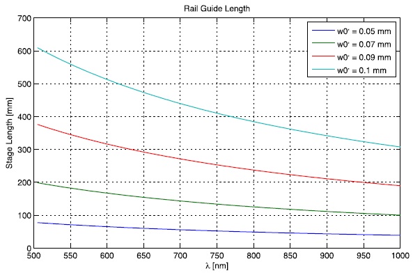
with a rail length of 5 times the Rayleigh range. To reduce the rail guide length, a right angle prism has been used as retro-reflector (Figure 5): the prism translation doubles the beam path, allowing space saving for the apparatus.
6. The final system
The conceptual scheme for the use of the apparatus is presented in Figure 10. The final system was built using off-the-shelf components, with special care to the affordability of the apparatus.
In addition to those listed in Figure 9, based on the described simulation and design criteria, the following components have been chosen:
-monochrome CMOS sensor DCC1545 from µ-Eye with 1024x1280 square pixels with side 5.2 µm, operative λ = 400 ÷ 800 nm; -biconvex lens with diameter 25 mm and focal length f = 500 mm; -micrometer rail guide with 600 mm of travel length.
The developed setup is transportable (less than 5 kg).
In a real application it is very difficult, even impossible, to move the laser source to adjust the beam path to match a determinate trajectory. The external laser beam is received by aligning optics and redirected on a predetermined trajectory along an optical track in Figure 9.
The CAD model of the apparatus, realized with Dassault Systèmes (2011), is shown in Figure 9 and commercial components are listed and described below.
The laser to be tested should be placed in the free space between units (1) and (2), facing the upper mirror (2u). Any external laser can also be tested, if it can be directed to (2u). High power lasers up to 1 kW can be characterized using a beam splitter.
The elements (2u), (2d), (3), (4), (6) compose the aligning optics. The beam travels through the air from (1) to (10), following an optical track formed by (2), (3), (4) and (7). The mirrors of the periscope (2) and the kinematic mirror (3) can be moved to align the beam to the correct path marked by the apertures (4) and (6). Before the beam strikes the prism it is focalized by a convex lens (4). The prism position is controlled by a micrometer rail guide (8s) with 50 µm resolution. The prism is supported by the translation stage (8) on the rail guide (9), allowing the movement of the prism along the propagation axis and the variation of the scanned section by the camera (10).
7. Beam characterization software
The measuring process is controlled via PC, with image analysis software implemented using the sensor software libraries Thorlabs (2010).
Two software modules and interfaces are available:
camera setting (exposure time, gain, …) and image acquisition (Figure 13).
image analysis to output parameters
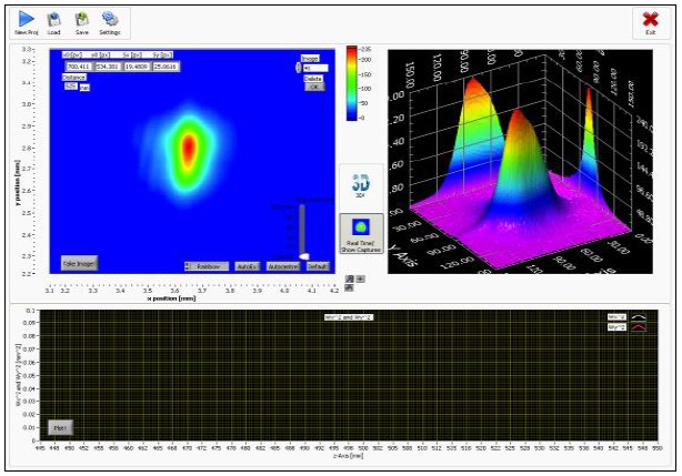
Figure 13 Interface of the acquisition module. Real image (top left) and 3D view with projections (top right). Preview of the propagation functions Wx(z) and Wy(z) estimated from a single image at each position.
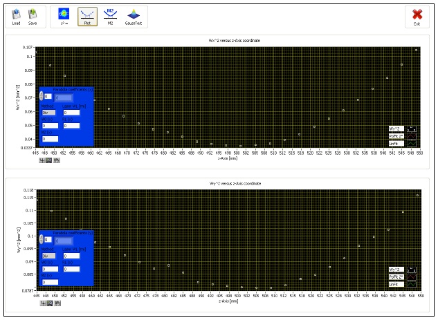
The image analysis module (Figure 14) processes the images extracting the beam radii and reconstructing the propagation functions W x (z) and W y (z) estimated from multiple images at each position (between 5 and 10). The two methods in Table 2 are available to estimate the beam parameters and to calculate M 2. Multiple images reduce the background noise and increase accuracy but take about 200 ms per image.
The total procedure including manual positioning takes about 10 minutes.
Figure 15 and Figure 16 describe the procedures for the image acquisition performed with the acquisition software (Figure 13).


Figure 16 Autoexposure procedure. This procedure automatically sets the exposure time to avoid image saturation, (max pij < 255). procedure. Multiple images are stored at each position.
For each position, several pictures (default is 5) are taken and processed to measure the beam radius. Each image is obtained by averaging 5 frames to reduce noise. The whole procedure is detailed in Figure 15.
The exposure time is dynamically modified to prevent image saturation according to the scheme in Figure 16 to compensate the intensity increase with the radius reduction.
Special care must be taken to cleaning the optical elements (Figure 17).

Figure 17 Detail of a real laser intensity image. Diagonal waves (1) caused by the diffraction of the neutral density (ND) filter. Round interference fringes (2) caused by dust grains on the CMOS sensor.
To reduce risks of faulty images with fingerprints or dust, morphology operation with kernel radius of 15 pixels size provides an alarm.
8. Validation of the apparatus
A visualization of the laser beam propagation, associated with radii functions, is offered in Figure 19.
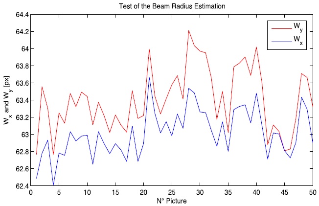
Figure 18 Measured beam radii on the two main axes from 50 images (cut=5). The mean and the standard deviation result [pixels]:

Figure 19 Laser beam sections along the beam path. The red line represents the squared radius variation. The images evidence that W0,x< W0,y.
The apparatus has been tested on a HeNe red laser and on a diode laser (Thorlabs, 2015). Tests on real images evidence a small relative standard deviation in Figure 18, coming from both the laser and the sensor in the radius estimation, if an adequate cutoff level is selected (Figure 21).

Figure 20 Relative standard deviation of the measured beam radius along the beam axis. The measurement error is less than 1.8%.

Figure 21 Effect of the cutoff level on the relative standard deviation. The beam radius is estimated over 50 pictures of the same section to evaluate the effect of the cutoff level on the mean and the standard deviation.
It can be noticed that for cut = 4 ÷ 9 the relative standard deviation is lower than 1% of the measured beam radius.
A statistical analysis to estimate the variance of the measured parameters (M 2 and W) from different data presents a low variability (Figure 20).
The radius propagation curves obtained with the apparatus show the expected parabola behavior (Figure 22). The M 2 x values for the diode laser are consistent with the ones available in the literature.
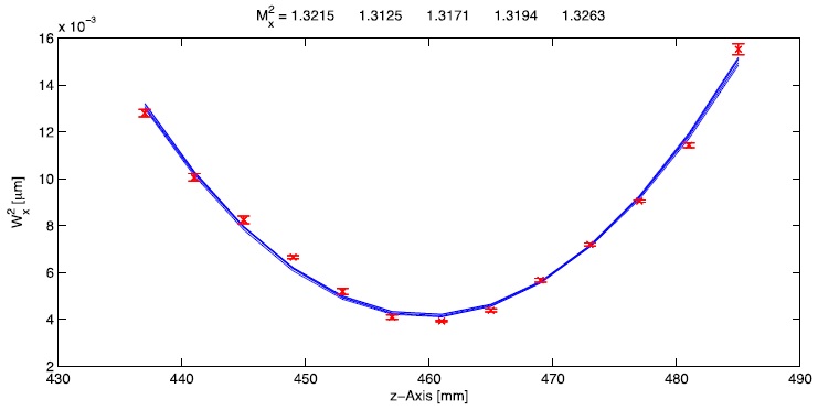
Figure 22 Radius propagation values and polynomial fitting (blue) from different data sets with error bars (red) indicating the mean and the standard deviations of measures and corresponding Mx 2 parameter values for the diode laser Thorlabs (2012).
9. Conclusions
The design and the realization of a beam propagation analyzer (hardware and software) have been presented. The M 2 and other relevant parameters measured by the apparatus have been characterized.
A camera sensor model has been proposed to estimate the minimum measurable beam radius (beam waist) to design the noise filter. The moment-based radius assessment is independent on the absolute intensity and distribution of the laser.
Current uses of the developed setup are laser beam characterization and staff training. Experimenters and equipment designers can benefit of the described design. The equipment and the software can be easily integrated into an existing system. The proposed system can be an alternative, in both industry and laboratory, to the more expensive commercial measurement systems. The system evolution includes a motor driven axis for mass production measurement; attenuating filters could be fitted if necessary in case of lasers exceeding the sensor power.

