


 text new page (beta)
 English (pdf)
 Article in xml format
 Article references
 Send this article by e-mail
 Cited by SciELO
  Similars in
SciELO
Similars in
SciELO 
 Permalink
1. Introduction
In recent years, more and more AUVs have been used for different researches on zones near the sea surface. When an AUV operates in this environment, significant oscillation disturbance due to waves will affect its motion Ochi (1998). Therefore it is necessary to carry out filtering techniques to counteract the undesirable effects of the waves on the control systems. Even when in deep water, an AUV has continually to come near the surface to look for satellite fixes for the purpose of navigation. A number of articles have explicitly addressed the depth control problem of submarines in a shallow wave perturbation environment Dantas, da Cruz and de Barros (2014), Qi, Feng and Yang (2016), Park, Kim, Yoon, and Cho, (2016).
In modern Dynamic Positioning (DP) and Autopilot Systems for marine vessels, the terminology low-frequency (LF) is used to refer to the states corresponding to the motion due to the action of the actuators and on the other hand, wave-frequency (WF) states represent the wave-induced components Fossen and Pérez (2009) and Shi, Shen, Fang, and Li (2017). For years, various techniques for wave filtering were investigated, including lowpass filtering, notch filtering, and dead-band techniques. These filters had limited success when high-gain control is required, which affect the performance of the DP system. Filters that exhibit better performances are those based on vehicle model and a wave induced motion model combined within an observer. For these purposes, the Kalman Filter is the preferred observer but it is computationally more intensive and the tuning procedure is difficult because a priori information of the process and measurement noise covariance is required Fossen (2011). Examples of wave force compensation by using a Kalman Filter framework are shown in Fossen and Pérez (2009), Wirtensohn, Schuster and Reuter (2016), Rigatos, Raffo and Siano (2017). In Dantas et al. (2014) the wave disturbances on the diving plane were filtered away by a shaping filter fitted to the sea spectrum and the sensor signals were integrated by an Extended Kalman Filter (EKF). In the work Wirtensohn et al. (2016), an Unscented Kalman Filter for performing disturbance estimation and wave filtering is investigated. Nonlinear passive observers also have been used to estimate parameters of the waves Refsnes (2007) and Belleter, Galeazzi and Fossen (2015). In general they are difficult to tune due to the number of parameters involved and the global stability is not guaranteed in all cases.The principle of combining inertial and depth measurements within a nonlinear observer has also been used for submersibles in Schmidt, Raineault, Skarke, Trembanis, and Mayer (2010).
In recent years, more advanced techniques have been reported, increasing the use of nonlinear sliding control among all of them. Despite of the fact that sliding mode controller is widely used in robot controlling, it is very sensitive toexternal disturbances and uncertainties in the models. When AUV performs the DP under the wave disturbance, the accuracy of the sliding mode controlling will be affected, and the chattering problem will appear. Therefore, a chattering suppression method or a disturbance observer need to be always added in order to eliminate the high-frequency control action inherent in a conventional sliding-mode controller. Several researchers have put forward different approaches to reduce this chattering phenomenon. Concerning marine applications, it is used in Xu, Du, Hu, and Li, (2014) a backstepping sliding mode controller with an adaptive term in combination with a disturbance observer for the compensation of the control law. Under the same principle, Du , Hu, Krstić, and Sun (2018) design a new adaptive control law for DP of ships, and an observer is inserted as additional element for handling disturbances.
Chattering is a harmful phenomenon because it leads to low control accuracy, high wear of moving mechanical parts, and high heat losses in power circuits, it was the main obstacle for its implementation in the vehicle under study. The different ways to eliminate chattering may take the cost of reducing DPs robustness with additional implementation complexity.
This article aims at the problem of wave disturbance rejection during the AUV motion in the diving plane. The solution proposed is quite different from these mentioned before. It is a passive observer based on linear models for depth/pitch response of the vehicle and a second order wave transfer function approximation, resulting in an easygoing filter. Following this idea, an observer was previously implemented in the embedded hardware of the same AUV for heading filtering Garcia-Garcia, Valeriano-Medina, Hernández, and Martínez (2012) and it was tested in many sea trials with excellent results. To illustrate the performance of the filter and the effects on the measurements and the actuators system, simulating results using MATLAB/Simulink are presented, as well as experimental validation based on real data obtained during a sea trial. The waves approximation used is similar to those proposed by Fossen and Pérez (2009) for surface dynamic positioning and Garcia-Garcia et al. (2012) for heading filtering. In comparison to the work of Dantas et al. (2014) they use two serial second-order transfer functions to represent the wave vertical displacement. The main feature of the algorithms developed for the vehicle under study is that they were computationally very light, due to the low cost hardware architecture of the vehicle. According to this, the linear observer designed is very easy to implement and less expensive from a computational point of view.
This paper is arranged as follows: Introduction, followed by the principal specifications of the vehicle under study in Section 2. The AUV motion modeling in the vertical plane and the model used to represent the wave induced motion are shown in Sections 3 and 4 respectively. Process for the observer design and tuning is showed in Section 5. Then, AUV depth and pitch control scheme is discussed in Section 6 followed by simulation results with the 6-DOF mathematical model of the vehicle and real data obtained during a sea trial. Finally, Section 7 concludes this work.
2. Description of the system
The latest design for submersible vehicle developed in cooperation between the Cuban Hydrographic Research Center (HRC) and the Group of Automation, Robotics and Perception (GARP) is called HRC-AUV. The primary envisioned missions of the prototype are environmental surveying andoceanographic data acquisition in coastal zones. Therefore, the vehicle is designed for small depths and medium endurance until depths lower than 10 meters. The length of the vehicle is approximately 9.5 m, has a diameter of 0.8 m and nominal cruising speed 1.9 m/s. The HRC-AUV uses a single main thruster for propulsion, steering and depth are controlled by two control rudders placed at stern and electrically driven. Fig. 1 shows schematically the hardware items comprised in the last version of the system after an update in 2014 Martínez et al. (2013).

The computational units are based on a PC-104 industrial computer, model PCM-3362 from Advantech and one embedded system based on two DsPIC 33FJ64 from Microchip. These two units share the data acquisition from sensors and the navigation/control tasks. The principal sensors installed in the AUV are:
○ Inertial Measurement Unit (IMU): MTi-G digital sensor from XSens Corporation. For accurate real-time attitude, orientation and absolute position of the vehicle. It is used only for surface or near the surface navigation to correct the INS solution.
○ Fluxgate compass: AA002803R from Vetus Company, analog sensor. Used to aid the INS solution.
○ Pressure sensor: Cerabar T PMP 131 from Endress+Hausser, analog sensor. Used to determine the operation depth of the AUV (conversion from pressure to depth). Used to improve the INS.
○ Battery level: Analog sensor. Estimates the status of the battery based on voltage and current levels.
○ Leak: Digital sensors located inside of the hull in order to detect any water leakage.
○ Rudders angle: MLO-POT-225-TLF from Festo, analog sensor. Provides the true position of the rudders.
○ Thruster rpm: Digital sensor. Provides the revolutions of the propulsion thruster.
3. AUV modelling
Six degrees of freedom (6-DOF) refers to the freedom of movement of a rigid body in a three-dimensional space. Consequently with this, the motion of a submarine at sea has the six degrees of freedom described as:
-Translation: Moving up and down (heaving), moving left and right (swaying) and moving forward and backward (surging);
-Rotation: Tilts forward and backward (pitching), swivels left and right (yawing) and pivots side to side (rolling).
The HRC-AUV moves at low speed of 1.9 m/s thus the rotation of the Earth can be neglected and the Earth-fixed reference system can be considered as an inertial frame and a North, East, Down (N.E.D.) the navigation frame. Fig. 2 depicts the coordinate systems and the definition of translation and rotation variables used. In addition, the nomenclature used to represent the position, velocity as well as forces variables of the HRC-AUV is shown in Table 1, which is the recommended notation used on maneuvering and control of submarines according to the standard SNAME (1950).

Table 1. Notation used forHRC-AUV modelling.
| DOF-Motion | Forces | Velocity | Position |
|---|---|---|---|
| 1-surge |
|
|
|
| 2-sway |
|
|
|
| 3heave |
|
|
|
| 4-roll |
|
|
|
| 5-pitch |
|
|
|
| 6-yaw |
|
|
|
3.1 General nonlinear vehicle model
In this section, we summarize the six-DOF non-linear dynamical model used to derive the proposed one-DOF linear model employed for the observer design.
To navigate properly, a good and accurate controller is necessary that's why a mathematical model of the AUV is needed. The general structure of the nonlinear model used here comes from Fossen (2011). He suggests that the general motion of an AUV can be written in the Body-fixed frame as:
Where
Several of the parameters for the model (1)-(2) were estimated from the vehicle's geometric and inertial data. Others, like those associated with the viscous damping and the control inputs, were estimated through experimental tests. Details of the experiments and validation of the general nonlinear model for the HRC-AUV can be found in Valeriano-Medina et al. (2013). This general nonlinear simulation model, including the effects of waves and ocean currents is used in this paper to validate the proposed observer for wave filtering.
Moreover, when automatic depth control is designed, it is only necessary to consider a model and perform wave filtering for depth and pitch degrees of freedom Fossen (2002) and Peñas (2009). In order to see its practical use, section below describes the linear dynamic model of the HRC-AUV in the vertical plane used in the wave filter.
3.2 Linear depth/pitch model
The general dynamics equations (1) and (2) of an AUV are complex and highly nonlinear, especially when it is subjected to environmental disturbances such as ocean currents and waves Faltinsen (1990). In conventional designs of observers, it is common to simplify the nonlinear dynamics of a system to linear dynamics about an operating point to obtain the transfer functions of the system Qi, et al. (2016). In De la Cruz, Aranda and Girón (2012) is suggested that the 6 DOF model of an underwater vehicle can be divided into four noninteracting (or lightly interacting) subsystems for speed, steering, diving, and roll control. Observers can be, in turn, designed for each subsystem separately. In Fossen (2011) linearized models of the vehicles are used to obtain the transfer function for steering and pitch controllers.
The depth kinematic relationship is obtained if it is assumed that the variables
Considering the Coriolis, centripetal and damping terms and if the forward speed is stable such that
Besides, if the pitch and depth loops become independent, it is possible to express
From Equations (1)-(2) the following relationship is obtained:
On this basis the transfer function between the stabilizing fins angle
Moreover, the relationship between the pitch angle
From Equations (7) and (8) are obtained the basics LF expressions for depth and pitch observer design, as:
Where:
Table 2 contains the terms used in the linear longitudinal model (9). These parameters were estimated from the geometric and inertial data of the vehicle as well as by means of experimental tests for the viscous damping and the control inputs; details can be found in Valeriano-Medina et al. (2013).
Table 2. Summary of HRC-AUV estimated and identified parameters.
| Term | Description | Value |
|---|---|---|
|
|
|
|
|
|
|
|
|
|
|
|
|
|
|
|
|
|
|
|
|
|
|
|
4. Wave disturbances modelling
Environment disturbances poses a great challenge in the control design for underwater robots. In practice, when an AUV operates in a shallow water (SW) area, significant disturbance due to irrotational wave will affect it Liang, Liu, Ma, Hirakawa, and Gu (2016). The SW area is defined as water depths from 40 feet to 10 feet. These disturbances are mathematically modeled in the following subsections to include it in the observer.
4.1 Surface waves and empirical spectra
Wind waves are generated by wind transferring energy from the atmosphere to the ocean's surface. Wind fluctuations cause water to rise above the equilibrium surface level Ochi (1998). The restoring force of these waves is gravity, hence they are called surface gravity waves and travels along a parallel channel described on Fig.3.

The
With
When
It is common to describe statistically the sea surface by the ocean wave spectrum
Various authors suggest that
Where
According to the Expression (15), a demonstration of how the Jonswap spectrum of surface waves attenuates with depth is shown in Fig. 4.
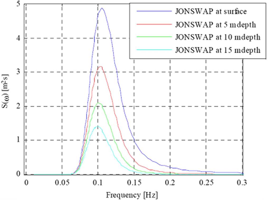
The area under the spectrum is equivalent to the energy of the waves. In shallow water, there is almost no attenuation with depth Park et al. (2016). It shows that even for more than 15 meters depth the surface wave effects are present Jalving (2007). Considering that the HRC-AUV will navigate at an average depth of about 5 meters, the mistake can be significant, hence the vertical position must be filtered out.
4.2. 2nd-order wave transfer function approximation
Because of the oscillatory motions that they generate, surface gravity waves can be reasonably well described by a linear analysis. A second-order, noise-driven filter is usually preferred by ship control systems engineers for modeling wave-induced motion due to their simplicity and applicability Shi et al. (2017). In this sense, it is common to write the wave amplitude
Where
Where:
In the Expressions (17) and (18),
Integrating both sides of the Equation (19)
and changing variable
Whose state-space form used in the observer design is defined as:
5. Observer design
The main purpose of the observer or state estimator is to reconstruct the unmeasured
5.1 Observer structure and tuning procedure
To obtain the observer equations, injection terms must be added to the dynamics Equations (17) and (22):
Where
Making use of the notation
Where:
Moreover, the characteristic equation of the error dynamic presented in (27) can be found by
Where
6. Results achieved
No reports were found in the literature of the application of this method to filter depth and pitch measurements for AUV, which is new in that sense. To demonstrate the performance of the proposed observer, simulation study is carried out using the six DOF simulation model of the HRC-AUV obtained in previous research that includes the effects of the environmental disturbances Valeriano-Medina et al. (2013). As depicted in Fig. 5, the control diagram consists of a dual loop control methodology with an inner pitch control loop and an outer depth control loop, which is commonly used in AUV depth control. The depth controller generates a desired pitch angle, which becomes the input to the pitch control loop. The pitch controller is a P-D with gains

6.1 Results using simulated data
With the goal to recreate the operation conditions of the HRC-AUV, the first simulations were performed with parameters of the waves corresponding to the sea behavior predominant on coastal zones in normal conditions. The amplitude of the pure sinusoid wave-induced motion is limited to 1.2 m. In addition, the wave model damping ratio is fixed to
Table 3. Description and classifications of sea states.
| Sea state code | Wave height (m) | Wave period (sec) |
|---|---|---|
|
|
|
|
|
|
|
|
|
|
|
|
If it's considered a head sea, therefore the direction of waves
Having completely defined the passive observer begin to develop simulations. Fig. 6 shows the LF depth observer output compared with the perturbed signal when the system receives a step variation of 3 meters at t=0. In this observer, further filtering of depth measurement is also filtered the pitch rate because both measurements are used in the control strategy implemented in the HRC-AUV. In that sense in Fig. 7 is shown the effect of filtering pitch rate, signal to be feedback to the inner loop of the cascade scheme used.


In addition, Fig. 8 shows the oscillatory behavior of the controller output due to wave induced motion in the vertical plane, variations that are considerably reduced when the signals used by the controller are filtered.

It is seen from the plots that most of the 1st order waves disturbances are filtered out, resulting in smooth estimates of the depth and pitch rate. Hence, the feedback controller should not be too much affected by the rough sea condition.
6.2 Robustness evaluation of the proposed algorithm
The robustness of the observer should be analyzed in different conditions such as: uncertainties in the vehicle model and changes in sea conditions. Finally, the design is completely robust only if the filter tuning is capable to support some variations in the 6 DOF vehicle model parameters and waves parameters.
For testing variations due to vehicle model changes, the parameters
Table 4. Parameters variationsfor the robustness evaluation.
|
|
|
|
|
|
|---|---|---|---|---|
| Test-1 | X | X | - | - |
| Test-2 | - | - | X | X |
| Test-3 | X | - | - | X |
| Test-4 | - | X | X | - |


In addition to the previous evaluation, variations in the dominating wave frequency used in the observer also are evaluated, which represents changes in sea states 1 to 3 according to Table 3.


As it is possible to discern, the results of the tests are quite similar to the one presented on Fig. 6 and Fig. 7, experiment in whichwas assume a total knowledge of the models used in the observer design. Therefore, it is possible to conclude that the wave filter based on linear observer is capable of assuming these model changes and of maintaining the desired performance within a limited range.
6.3 Results using real data
Prior to implementation of the filter, several simulations were conducted to assess the performance of the observer developed with real data. Instead of, specific sea-trials navigation data from a survey mission performed few months ago were used. During the sea trial, the vehicle was operated at constant heading and low depths, under the influence of strong wave action. Figs. 13 and 14 show some of the practical results obtained during depth changing maneuvers, along with the results of simulations obtained with the linear passive observer.


At the beginning of this maneuver the HRC-AUV was at sea surface; then the depth controller was switched on and a command to dive to 2 m, 3 m and 4 m depth was given.Moreover, Fig. 15 exhibits the changes in the control signal to the rudder (elevator). A better performance of the depth control is evident; the WF motion caused by the ocean waves is removed and the actuator system receives only the desired control action. The transient response obtained including the observer included is similar as the real response.

In Table 5 a comparison among statistical values of the rudder control signal is displayed when the LF observer outputs are used in the depth control. The wave frequency components are filtered out, reducing energy consumption and increasing the life time of the actuators.
7. Conclusions and future work
Application of a passive wave filter algorithm for AUV navigation in the diving plane was presented. The proposed strategy enhances the quality of the AUV depth/pitch control significantly, reducing the amplitude of oscillations generated by the ocean waves, allowing the AUV to navigate properly in shallow zones or close to the surface.
Several simulations to support the expected results were given, including sea trial data. It has been shown that both the LF depth and pitch rate of the vehicle can be computed from noisy depth measurements, resulting in smooth and precise estimates. The wave filter is relatively simple, easy to tune and consequently feasible to implement in the embedded hardware for real-time operation.
Future work aims to expand the methodology used here, to the 3 degrees of freedom horizontal model and developing a wave encounter frequency estimator for online tuningof the observer gains.

