


 nova página do texto(beta)
 Inglês (pdf)
 Artigo em XML
 Referências do artigo
 Enviar este artigo por email
 Citado por SciELO
  Similares em
SciELO
Similares em
SciELO 
 Permalink
1. Introduction
The trajectory planning and obstacle avoidance of autonomous are research topics currently in full development (Alajlan & Koubâa, 2016; Fakoor, Kosaři, & Jafarzadeh, 2016; Medina, Camas, Vazquez, Hernández, & Mota, 2014; Varkonyi-Koczy & Bencsik, 2010). Numerous algorithms have been produced; but initially these were for mobile robots deployed in environments with well-defined obstacles. Among these algorithms, roadmap, cell decomposition, Voroni diagrams, and Potential Fields methods, can be highlighted (Li & Canny, 1993; Peng. Tang, Xin, Wang, & Kim, 2014; Perez, Godoy, Villagra. & Onieva, 2013; Voronoi, 1991). However, the growing need for designing and implementing mobile robots capable of orienting themselves while exploring their surroundings (Alves, Marcharet, & Campos, 2009; Goerzen, Kong, & Mettler, 2009; Rullan-Lara, Salazar, & Lozano, 2011; Yang, Gan, & Sukkarieh, 2009) has led to the advance of several techniques for the generation of online trajectories. These techniques are based on deterministic elements such as the A* Algorithm (Valenzuela, 2009), and on random elements like the Rapidly-exploring Random Trees (RRT) algorithm (Alves et al., 2009). The conditions of the problem determine the technique to be used.
The need to generate automatic and dynamic routes gives rise to techniques in which a robot perceives and understands its surroundings, locating itself in its habitat thanks to its sensors, localization algorithms, and controllers. Accordingly, Simultaneous Localization and Mapping (SLAM) incorporates basic probabilistic techniques for the correct handling of information. In addition, the simultaneous automatic localization and mapping of the surroundings approach provides the robot with the information required for using some method to generate its route (Lemus, Díaz, Gutiérrez, Rodríguez, & Escobar, 2014; Nuchter, Surmann, Lingemann, Hertzberg, & Thrun, 2004; Thrun & Montemerlo, 2006); therefore, the generation of efficient trajectories is a matter still under study.
2. Harmonic potential fields by means of the method of panels
Although widely accepted in the community, the potential fields method has problems with local minima; therefore, different heuristic techniques are used to rescue a vehicle after a local minimum has been identified (Julia, Gil, Payá, & Reinoso, 2008). A variant of this method is known as harmonic potential fields (Daily & Bevly, 2008; Masoud, Ahmed, & Al-Shaikhi, 2015; Padilla, Savage, Hernandez, & Cosío, 2008; Shi, Zhang, &· Peng, 2007), which uses a model of irrotational flow that lacks local minima, with the vector field velocity of this fluid denoted by V. However, our interest is focused on this fluid's gradient, as shown in (1):
Where:
From (2) it is deduced that the fluid's velocity can be written as:
where ϕ is a scalar velocity potential. On the other hand, when the fluid is incompressible, the velocities field must satisfy (4):
Now, substituting (3) into (4) we obtain:
where
2.1 Properties of harmonic functions
The properties of any harmonic function are four:
i. Superposition. The total potential can be obtained from the linear combination of different harmonic-potentials.
ii. Mean value. A potential function, which is harmonic at the center of a circumference ϕ(x c1 ,x c2 ), will take a mean value of the total potential defined by (6):
This property implies that the value of the potential at the center of a circumference or located in an arbitrary place within it equals the mean value of the integrated potential around that circumference. Additionally, this property is independent of the radius r and depends only on the function being harmonic within the circumference. In the three-dimensional case this property maintains and is expressed by (7):
iii. Maximum Potential. The maximum of a harmonic function occurs in the limits of the singularities when the potential tends to infinity.
iv. Minimum Potential. The minimum of a harmonic function occurs in the limits of the singularities when the potential tends to infinity.
2.2 harmonic potential in two dimensions
A symmetric harmonic function does not depend on angular terms, but rather on the distance to the origin r, i.e., ϕ=ϕ(r). In general, for ท-dimensions the expression of Laplace's equation in spherical coordinates can be written as:
where C is a constant. For two dimensions, the harmonic-function can be represented by means of (9), while for n-dimensions the harmonic potential equation is (Fahimi, 2009):
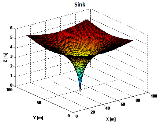
In hydrodynamics, a harmonic function with spherical symmetry of type (8) and (9) is called a source or sink depending on the sign of C1 or C 3 . In this paper we will consider a source/sink the equation defined in (11), depending on the sign of λ, which will be called source when λ<0 and sink when λ>0.
The distance to the goal r can be decomposed into Cartesian coordinates, as described by (12) and Figure 1, considering the position of the vehicle and the goal.
2.2.1 Panels
Figure 2a schematizes a point in space defined as an obstacle, which implies that the constant of (11) is positive (/1 > 0). Generalizing that point obstacle into a panel of the shape in which the obstacle is perceived by the vehicle, as schematized by Figure 2b, (13) is obtained, which models the behavior of the potential. In this way, any obstacle will be defined in the Cartesian plane as a panel of length l.
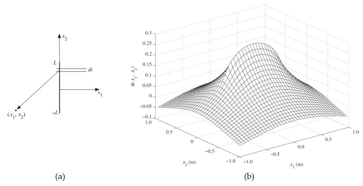
Once the obstacle has been defined, the gradient (ϕ panel ) is determined to establish the potential flow that the vehicle must follow in the Cartesian plane defined by (14).
2.2.2 Uniform potential flow
Other function used to construct the harmonic field potential is uniform flow potential, which varies linearly toward the objective point. This potential is used to ensure the convergence of the flow toward the goal by means of the singularities presented in (11). The uniform potential is defined by (15), where U represents the force constant of the uniform flow, and is the angle formed by the initial position of the vehicle and the goal, according to (16) .
2.2.3 Multi-Panels
Any obstacle can be approached as an x-panel polygon containing the obstacle inside (see Figure 3).
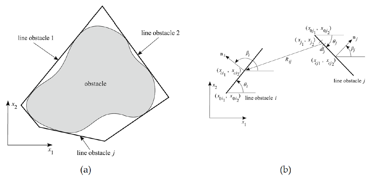
Under this premise the harmonic field potential is defined as the linear combination of the attractive, repulsive (panels), and uniform field potentials, so the resultant net potential is represented by (17):
Where R ij is the distance between the central point of where i and a differential point dlj of panel j, and λj corresponds to the repulsive force of panel j, whose value is obtained in a way that is adaptive t the initial conditions (Fahimi, 2009) Therefore, the net gradient of the harmonic field potential will be defined by:
3. A* algorithm
The A* algorithm is a search algorithm that allows finding the lowest cost route between two points based on a given evaluation function. It is classified as a search algorithm in graphs, since it provides robotized vehicular mechanisms (virtual or implemented) with an autonomous navigation system (Rolf, 2004).
This algorithm is in charge of finding the route with the lowest cost between a point A and a point B by using a heuristic function which consists in an approximation between the real distances of A and B.
The heuristic function f(x) is the result of the sum of two other functions: one that indicates the cost of the route that has been taken to a given node, which is represented as g(x), and other that gives an estimation of the distance between the point or node at which the robotized vehicular mechanism is with respect to the goal, represented as h(x). Therefore, the heuristic evaluation function is the result of the linear combination of h(x) and g(x).
3.1 Definition of the heuristic evaluation function
Considering the heuristic function ƒ (x) = h(x) + g(x), it is found that:
where constant Cost represents the explicit value of moving from the present point to the following node in some given direction, which if not specified will be taken as equal to one, because in this way a uniform distribution is assumed; node x , y represents the Cartesian coordinates of the current node and Objetive x,y represents the coordinates of the goal or objective (Tariq, 2008). This heuristic measurement is known as the Manhattan distance (Jönsson, 1997).
On the other hand, we have that g(x) is defined as:
where α corresponds to a constant whose value fluctuates between 0 and 1, defined for the problem to be faced, which will determine the branching degree of the algorithm. In addition, g(x)n-1 represents the g(x) value of the previous parent node. The pseudocode that defines the A* algorithm is presented in Table 1 (Valenzuela. 2009).
Table 1 Pseudocode of the A* algorithm.
| [1] | Initialize OPEN list |
| [2] | Initialize CLOSED list |
| [3] | Create goal node; call it node_goal |
| [4] | Create start node; call it node_start |
| [5] | Add node_start to the OPEN list |
| [6] | While the OPEN list is not empty |
| [7] | { |
| [8] | Get node n off de OPEN list with the lowest f(n) |
| [9] | Add n to the CLOSED list |
| [10] | If n is the same as node_goal we have found the solution; returns Solution(n) |
| [11] | Generate each sucesor node n´ of n |
| [12] | For each successor node n´ of n |
| [13] | { |
| [14] | Set the parent of n |
| [15] | Set h(n´) to be the heuristically estimate distance to node_goal |
| [16] | Set g(n´) to be g(n) plus the cost to get to n´ from n |
| [17] | Set f(n´) to be g(n´) plus h(n´) |
| [18] | If n´ is on the OPEN list and the existing one is as good or better, then |
| [19] | discard n´ and continue |
| [20] | If n´ i son the CLOSED list and the existing one is as good or better, then |
| [21] | discard n´ and continue |
| [22] | Remove ocurrences of n´ from OPEN and CLOSED |
| [23] | Add n´ to the OPEN list |
| [24] | } |
| [25] | } |
4. Evaluation of algorithms performance in complex surroundings
The main objective of this work is to evaluate the performance of the two algorithms presented (Harmonic Potential Fields and A*) and select the one with the best performance for future implementation in a real mobile robot. Initially, this robot will not know its surroundings and will only get limited information about its environment by means of its sensors, which implies that it will have to trace the route dynamically from the starting point of the movement to its goal. To evaluate these algorithms, critical surroundings generated by the possible structures that the robot can detect in unknown environments are assumed, namely:
The selection criterion of the algorithm with the best performance is based on the shortest possible time to obtain the solution that allows the robot to reach its destination and the goal successfully.
4.1 Evaluation of harmonic field potentials using the method of panels in environments with local minima
4.1.1 U-shaped structural obstacle
When simulating a U-shaped obstacle -in the x-y plane-whose position is known by the robot, which starts its path from point (25,45) to finish at coordinates (25,5), the following trajectory is obtained:
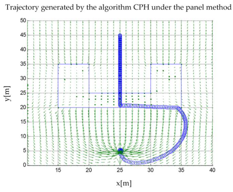
Fig. 4 Simulated trajectory of the robot faced with a บ-shaped obstacle with harmonic field potentials by the method of panels.
Figure 5 shows that the panel method is unable to solve the trajectory problem when faced with spatial configurations that generate a local minimum as strong as those formed by the U-shaped structures. In a more detailed way, Figure 6 shows the gradient of the generated harmonic potential.


To solve this problem, the authors (Wijs, 1995) and (Saudi & Sulaiman, 2012) propose using the Laplace limit conditions, i.e., the highest potential would exist in the map's edges, and mathematical operations will be performed to decimate the effect of local minima shown in Figure 6. However, conditions based on harmonic-potential fields have a high computational cost and, in general, are carried out off-line; therefore, the method is not adequate for use in future applications.
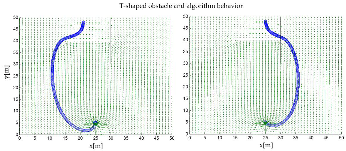
4.1.2 T-shaped structural obstacle
When developing a T-shaped structure, the harmonic potential field algorithm is capable of reaching the goal by evading part of the structure. Nevertheless, when having a look at the field flow, it is observed that the algorithm does not recognize the panel placed in a vertical position with respect to the x axis. creating the possibility of circulating and crossing that panel, i .e., the behavior of this algorithm with this kind of structures is not optimum. Furthermore, when different starting points are attempted, the algorithm diverges, thus confirming the previous idea, as schematized in Figure. 7.
4.2 Evaluation of the A* algorithm in structural environments with local minima
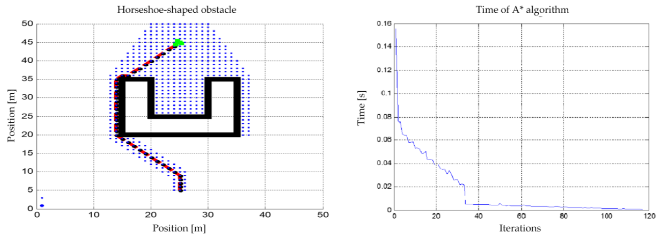
4.2.1 U-shaped Structural Obstacle
When the A* algorithm is exposed to a U-shaped structural obstacle, an absolute convergence from the starting point to the goal is seen, i.e., it is capable of recognizing the local minimum generated by the structure and developing a route that involves the smallest distance cost according to the stated heuristic. Figure 8 shows the evolution of the algorithm and the time that it takes to find the goal while the vehicle is in motion. In the following simulation it is seen that the maximum time taken by the algorithm to detect the goal is 0.16 seconds,
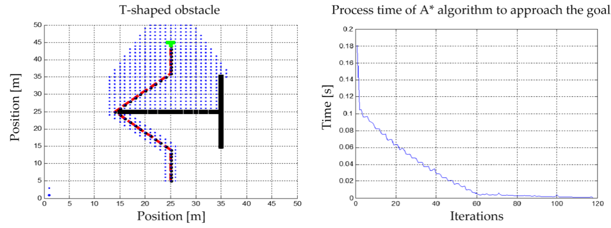
4.2.2 T-shaped structural obstacle
which is achieved in the first iteration. After this, the required time drops sharply as the vehicle moves toward the goal.
When faced with a T-shaped structural obstacle, the algorithm again converges with the goal when a structure is detected and a route is generated that allows the vehicle to evade the obstacle. Also, when the starting point is modified the algorithm exhibits no problems and once again it finds the destination point.
The maximum time taken by the algorithm to generate the route toward the objective is 0.180 seconds in the first iteration. Then, as the vehicle approaches the goal, the algorithm decreases its process time linearly, as shown in Figure 9.
5. Selection of the algorithm
The results from the algorithms performance obtained in Section 4 are shown in Table 2.
Table 2 Results of the performance of the algorithms.
| Algorithm | Local minima present | Reaches the goal | Maximum calculation time (seconds) | Goes over the obstacle | ||
|---|---|---|---|---|---|---|
| U | T | U | T | |||
| A* Algorithm | No | No | Yes | Yes | 0.18 | No |
| Harmonic Potential Fields with method of panels | Yes | Yes | Yes | Yes | 5.5x10⁻⁶ | Yes |
Although the calculation process of the A* algorithm is much longer compared to that of the harmonic potential fields algorithm under the method of panels, it ensures the total convergence of the vehicle to the goal. However, the calculation process time increases exponentially depending on the size of the map. In view of these results, the A* algorithm is the one that will be used for the implementation of a real exploring vehicle.
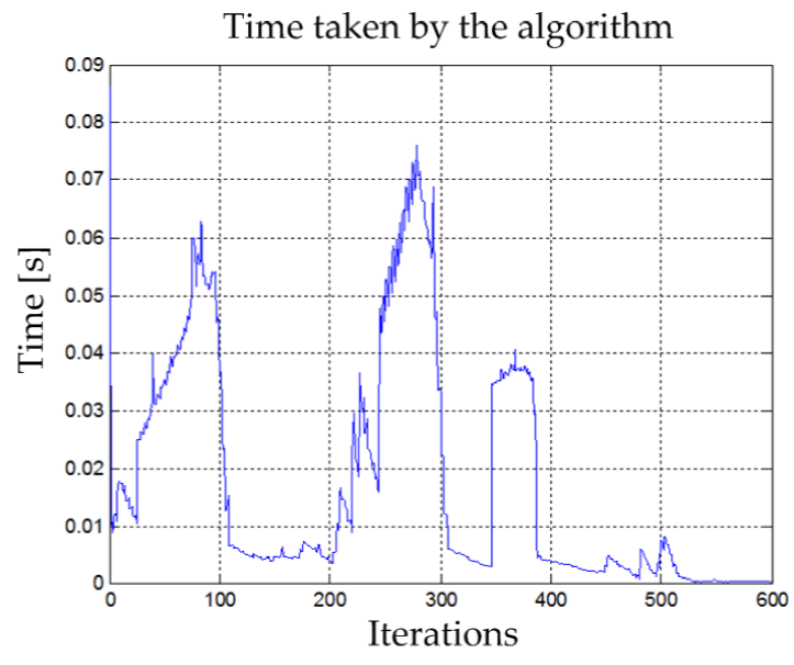
When complex surroundings with multiple structures that generate local minima are simulated to trace the virtual route that the vehicle must follow emulating the robot's perspective, i.e., it is able to see the changing environment as it moves over the Cartesian plane, the A* algorithm is capable of finding the goal in a satisfactory way, regardless environment complexity, e.g., dynamic or static, as presented in Figure 10. The time taken by the algorithm to recalculate the new route after detecting new obstacles in the robot's field of view is shown in Figure 11. In this figure, the maximum time it takes the algorithm to calculate the route is 0.09 seconds for the first iteration in a map of 50 by 50 cells; then, as the robot moves and its vision of the environment changes, the process time varies dynamically.
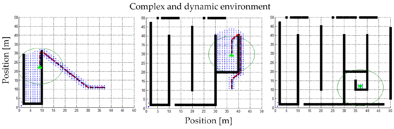
Fig. 10 Evolution of the vehicle's trajectory when faced with dynamic changes of the perceived environment.
Conclusions
This paper presented and evaluated the performance of two algorithms that allow a mobile robot to orient itself as it explores its environment, namely harmonic potential fields, by means of the method of panels and A*. In a previous study, the authors evaluated various methods for generating routes, such as visibility graphs, Voroni diagrams, cell decomposition, genetic algorithms, probabilistic padmaps, harmonic potential fields by the method of panels, A*, among others, finding that the last two algorithms yielded the best results due to their degree of convergence and robustness when faced with changes in the environment. To assess their performance, we assumed critical surroundings generated by the possible structures that a mobile robot could detect in an unknown environment (U- and T-shaped), considering the ability of the algorithms to find the objective point in settings with strong local minima as well as process efficiency, i.e., the time taken to find that point.
In Section 4 it was established that the harmonic potential field algorithm did not have a good behavior when faced with complex structures and non-point obstacles identified by the method of panels. In the บ-shaped obstacle, the potential gradient crossed the structure and provided the bottom part of the obstacle points to the objective, as shown in Figure 4. This algorithm was not able to distinguish clearly a structure orthogonal to the X axis, as it did not perform optimally when faced with non-point structures, as can be seen in Figure 7. However, the algorithm exhibited excellent performance in point obstacles located in an open space, i.e., without well-defined boundaries, completely converging with the goal. It must be pointed out that the time required by the harmonic potential field algorithm to generate the route is considerably shorter than that of its counterpart discussed in this paper.
It was determined that to solve the problem of divergence of the harmonic potential fields algorithm it was necessary to use Laplace limit conditions. However, this process must be carried out off-line, so it is not applicable to our problem because our robot initially will not recognize its surroundings and will only obtain limited information about the environment through its sensors, which means that the robot must trace the route dynamically from the motion starting point to the goal. The A* algorithm proved capable of supporting complex environments with strong local minima generated by dynamic and/or static structures. This statement is confirmed by Figure 10, in which the algorithm is tested in dynamic surroundings under constant change, as the robot can perceive its surroundings but limited to a few meters around, with A* determining the optimum route for the robot at each step.
Nevertheless, the A*algorithm has a high computational cost compared to the harmonic potential field algorithm using the method of panels. Moreover, when the size of the map increases, so does the algorithm's computing time. However, A* is capable of finding the goal as long as the environment conditions allow the transfer of the vehicle, making it possible to generate optimum dynamic routes across unknown surroundings according to the information obtained from the environment.
The criteria for selecting the best algorithm was based on the ability to find the point objective in environments with strong local minima. These local minima were solved by the two algorithms discussed, thus enabling the robot to overcome and/or get out of complex structures. Furthermore, the efficiency of the algorithms in the calculation process, i.e., the time needed by them to reach the objective point satisfactorily, was analyzed and presented, considering that the shorter the time, the greater the weighting for selection. In conclusion, the selected algorithm is A*.

