1. Introduction

Nowadays it is almost required to obtain the best results in any given situation in most areas of science. In this sense, optimization is a way to obtain such results.

Through the years, several optimization methods have been developed, which can provide better results in comparison with others, depending of the characteristics of each one. Most of these methods have been implemented in digital computers, and due to the high capabilities to process and manipulate data, computers have allowed a quick progress in the area of optimization.

Several commercial software packages that implement optimization methods are capable to plot a surface and find optimal solutions, but they focus exclusively on numerical solution without analyzing curves and surfaces interactively, therefore, limiting the interpretation of results. It is possible to find professional software with characteristics related to those implemented in the software described here, such as ^{MatLab© (2017)}; ^{Maplet© (2017)} and ^{Mathematica© (2017)}, but the acquisition of those packages might not always be justified, and often, the environment becomes complex due the wide set of tools that are available.

Besides, some developers use the capabilities offered by commercial software packages in order to build optimization tools, such as TOMLAB (^{Holmström, 1999}: Ríos & Nikolaos, 2013) and YAMLIP (^{Löfberg, 2004}). These tools, use MatLab to implement well-known optimization algorithms and also to develop new algorithms, each one of these have their own approach and scope. Another optimization tool, OPTI (^{Currie & Wilson. 2012}), which provides support to MatLab users, has also a collection of several solvers.

There are also public domain software packages that replace, in part, those expensive software packages and implement optimization technics, such as ^{Octave (2017)} and ^{Scilab (2017)}. Further options are optimization libraries, but they represent unfriendly environments for those users without programming training. Furthermore, all these software packages and libraries, require a broad knowledge related to a specific programming language or in other cases, the knowledge of particular statements. Thus, in some cases it is preferable to use a specific-application software.

A novel software package for optimization named OptimPlot is proposed to overcome the disadvantages mentioned above. Furthermore, OptimPlot is mainly addressed to researchers without knowledge of optimization algorithms and programming trends, who require the solution of an optimization problem in a simple way, and without the need of writing code lines.

The article reports the development of the new software package OptimPlot that includes the features of two applications that work independently (^{González-Palacios, Bernal-Martínez, & Aguilera-Cortés, 2009}: ^{González-Palacios, Peña-Gallo, &· Aguilera-Cortés, 2009}). Besides, OptimPlot incorporates features that provide an integrated and autonomous environment. Among them are included, the possibility of plotting several functions simultaneously in two and three dimensions; the introduction of the concept to consider one variable as a parameter that can be adjusted continuously to plot two-variable functions in a 2D environment; as well as the introduction of a pane control that allows the user to easily handle the graphical interface.

The software package is developed on a robust platform of software development, called ADEFID {ADvanced Engineering platForm for Industrial Development) which is a set of libraries. The ADEFID platform simplifies and enhance software development, since any application created with this platform contains by default a set of functions that facilitates the construction of the graphical environment, as well as functions that interact with the pointing device (^{González-Palacios, 2012}). Thereby, OptimPlot encompasses a graphical environment based on OpenGL and mathematical algorithms written in Visual Studio® C++ and structured with the object-oriented programming (OOP) concept (^{Horton, 2010}; ^{Latore, 1999}; Lemecker & Archer, 1998; ^{Stroustrup, 1997}; ^{Walnum, 1999}). These features allow the creation of a robust, efficient and flexible software. Several software packages, with research interest, have been developed on this platform, for instance, ProCart (^{Peña-Gallo, 2011}), which is focused to perform both on-line and off-line graphical motion simulations, as well as to control the motion of a cartesian manipulator.

Thus, OptimPlot is a specific application software providing a helpful graphical tool to analyze and optimize functions in two or three dimensions, with the advantage of an interactive operation while keeping the function plotted. The solution of an optimization problem can be done selecting different methods. Moreover, the user can navigate on the surface or curve to establish an initial point and find the optimal or critical point, which can be observed on the plotted function.

Another advantage of OptimPlot is the clear and full control on the algorithms involved in the main program. The user can properly operate the software with only a basic knowledge about the main optimization techniques. This way, the more the user is familiar with optimization techniques, the better OptimPlot can be exploited. Nevertheless, if the interest of the user resides exclusively on the visualization of the plotted function, no knowledge on optimization theories is required.

In summary, within engineering activities, scientists and students require graphical tools to be able to interact with plots of mathematical functions (in two or three dimensions). This interaction has different goals, for instance, visualize the behavior of a function, analyze its critical points, or in other cases the application of optimization techniques. OptimPlot was born then, to provide the support of performing these tasks in a simple and intuitive environment, thanks to the combination of the optimization theory with novel graphical user interface concepts introduced in this paper.

In Section 2, the software structure and the relation between the implementation of several classes are discussed. Section 3 is dedicated to present the main characteristics of OptimPloT. The description of the implemented methods to find critical points is carried out in Section 4. In Section 5 some examples are analyzed and solved with the application of OptimPlot.

2. The software structure

In order to simplify the use of the software, the required tools are encapsulated in two specific environments to analyze the given function: to analyze a single-variable function the 2D environment (2DE) is provided, and in the same way there is a 3D environment (3DE) to analyze a two-variable function, having each one its own characteristics.

The software developed is supported by the Microsoft Foundation Class (MFC). MFC is a standard library that provides an object-oriented wrapper to develop user interfaces with multiple controls and Office-style user interfaces. The principal MFC classes used in OptimPlot are CDocument, CView, CFormView and CDialog, the former with the Multiple Document option to improve the user interface flexibility. Therefore, the software is compatible with Microsoft Windows® operating system.

Some classes afforded by ADEFID libraries have been used to build the graphical structure of OptimPlot. Nevertheless, specific classes to manage OptimPlot were developed. In Fig. 1, the class diagram is shown, representing the general structure of OptimPlot, where the arrow symbol means "derived from". Referring to the Fig. 1, in the level of ADEFID classes there is a group, enclosed by a dashed box that supports the graphical interface, namely, CIpiGLDoc, CIpiGLView and CAdefidRender. Is possible to see that CIpiGLDoc and CIpiGLView are derived classes from MFC libraries.

Fig. 1 Class diagram of OptimPlot. 

Within the same ADEFID classes level, there is a set of classes specifically developed to support OptimPloT. This set, mainly contains algorithms to plot functions in two or three dimensions, as well as those algorithms required to optimize mathematical functions.

The purpose of the derived classes located at the OptimPlot classes level, is to create and manage the interface between the user and the software application.

2.1 About the main libraries and classes

CAdefidMDView and CAdefidMDDoc are basic classes in any ADEFID project because they are derived classes from CDocument and CView. The OptimPlot's main process resides in CAdefidMDDoc, whereas CSimulationForm class manages the user operations pane.

The main task of the CFunGenMachine class, is to interpret the function entered as string of characters by the user.

The CIpiGLView class is devoted to manage all window messages required to interact with the mouse and to perform the setup and initialization of OpenGL.

The IpiGUI library contains classes to support the graphical interface. This library is used as a base class to create the C3DPlot and CPlanarPlot classes, which were specifically developed to suit OptimPlot'ร needs. The former is applied to plot two-variable functions f(x, y), while the latter, to plot single-variable functions.

To provide an idea on the content on the above-mentioned classes, a piece of code of a function member is listed in Fig. 2. With the aid of the OpenGL capabilities, such as generating a surface applying linked strips of quadrilaterals to an ordered cloud of points, the C3dPlot::Draw3DFunction() function generates the surface of a three-dimension function. The pseudocode starts from the knowledge of the x and y range [x _min , x _max , y _min , y _max ] and the distance between points [Δx, Δy] of a given f(x,y) function. Results on the application of this function are appreciated along the manuscript (see Figs. 3, 7, and 10, 11, 12, 13).

Fig. 2 Pseudocode of the function that creates a surface 

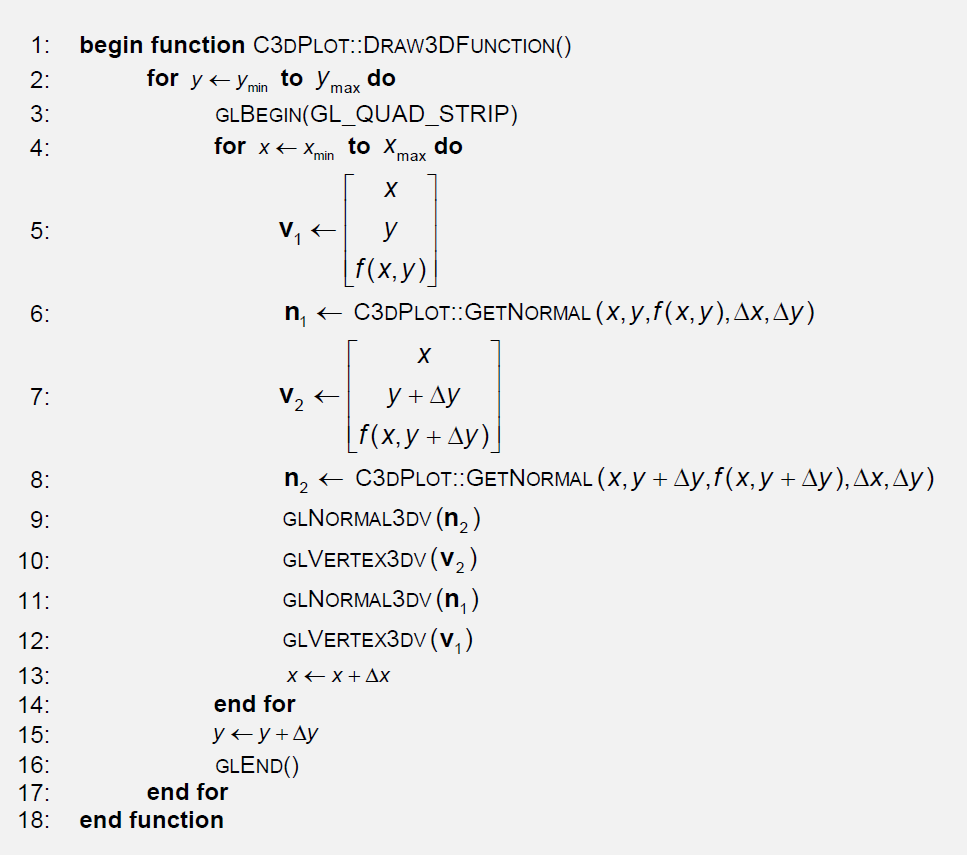
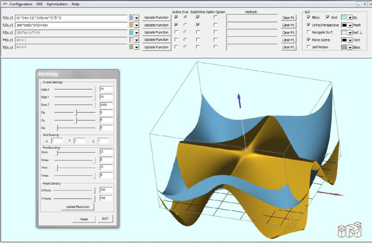
Fig. 3 The 3DE to analyze three-dimension surfaces. The plotted function in blue is given by (x12+x2-11)2+(x1+x22-7)2 and the other plotted surface is given by 300cos(xy/5) + 100. 

The purpose of CAdefidRender class is to render all the objects seen on the screen. It contains two virtual functions, namely, SetupScene() and RenderUScene(). The SetupScene() function creates the components of the scene, and RenderUScene() update the scene if any transformation take place. In this way, when the user manipulates the function (rotate, move, translate, zoom-in or zoom-out the scene) the function is not calculated, it is only called as a scene object, but only when the user makes a change on the function expression, SetupScene() is called to perform the corresponding calculations to update the object representing the function.

IpiOptim is an OptimPlot's library with several classes implemented to analyze mathematical functions. These classes are described in Table 1.

Table 1 IpiOptim library classes 

Class Name	Description
CBisection	Classes to obtain roots of a single-variable function, f(x)
CFalsePosition
CFixedPoint
CNewtonRaphson
CSecant
CGoldenSection	Dedicated class to the obtaining of critical points of a single-variable function.
CDavFlePow	Methods applied to get minimum values of a n-variable function.
CDirCon
CModMar
CStreepestDescent
COptimFunctions	A base class with virtual functions required to analyzed critical points.

OptimPlot has the property to read and to interpret the symbolic definition (as string of characters) of a mathematical expression. It is the CIpiMath class which provides this feature. This class analyzes the string of characters to build a graph without any more statements.

3. Main characteristics of OptimPlot

The OptimPlot philosophy is to provide an intuitive environment with easy handling, therefore, releasing the user from writing code lines. This way, the user focuses on the solution of the problem and not on how to operate the software.

Based on the statement above, the expression of a function is input as a symbolic form, using the conventional arithmetic operators, listed in order of priority: ( ), ^{^} , *, /, +, - ; and the default literals to be used as variables are x and у .

The user can input up to five functions simultaneously and decides whether to plot a single one of them or all by clicking on the corresponding Check Box Control. With the same idea, by means of a Radio Button Control, the user decides which of the displayed functions will be selected for evaluation on critical points. Furthermore, if any of the functions is edited, it is modified on the screen by pressing the corresponding Update button.

Although 2DE is devoted to single-variable functions ƒ(x) , it is possible to input functions of two variables ƒ(x, y), in which у is considered as a parameter with a given value specified by the motion of a Slide Control. This feature allows the user to interactively visualize the function'ร behavior while the parameter у changes from one value to another within a given range of x .

In order to make the use of OptimPlot more user-friendly, the graphical environment was developed so that it could be easily customized. The user can manipulate some graphical properties such as the function color, the background color and the surface representation (orthogonal or perspective) among others. In Fig. 3, a 3DE screenshot is shown, in which two surfaces are simultaneously plotted. Furthermore, in the same figure, the tools to handle the objects and the scene are visualized.

The change of the color function can be performed by means of the Color Button Controls, located next to the edit box. Other options are clustered in the GUI Group Box, as shown in Fig. 3. Some of these options are useful to change the objects color involved in the graph, such as Back Ground (BG), Mesh, Reference Lines (Ref. L.), Text and Block Plate (B. Plate). Other functions, are check box items that modify components of the graphical interface, as described below:

There are other options to interact with the objects and the scene, such as Dialog Windows to manipulate the environment parameters, moreover, the changes in these dialogs, affect instantaneously the plot environment. These dialogs can be accessed through the Menu Bar, which has three options, Configuration, GUI and Evaluate or Optimization depending if the application is 2DE or 3DE, respectively:

4. The optimization problem

The optimum seeking methods or mathematical programming techniques are useful to find the minimum of a function of several variables under a prescribed set of constraints; however, it is possible to find a maximum with the same techniques that were used to find a minimum performing some changes. The minimization of functions without constraints is obtained by the applications of these techniques.

The optimization methods implemented so far in OptimPlot, are the classical techniques commonly reported in the literature for unconstrained optimization problems, and they fall into the branch of mathematical programming techniques (^{Arora, 2004}; ^{Fletcher, 1987}; ^{Rao, 2009}).

The general mathematical programming problem can be expressed as: find the design vector X which minimize or maximize the function ƒ (x) :

where ƒ(x) : is the objective function and it is constrained by:

moreover, the values of the design variables (design vector components) are limited by:

where X _i , _m and X _i , _M represent the minimum and maximum value that the design variable can take, and these are called design constraints. The design vector which minimize or maximize the objective function is commonly called the optimal solution and is expressed as x*.

An extensive amount of options is available to solve the optimization problem. In many cases, the main limitation, is determining the adequate optimization techniques to solve the given optimization problem, several optimization methods are implemented for this reason.

4.1 The two-dimension optimization problem

The problem is concentrated in a single-variable function, у=f(x) Thus, the function to be analyzed has critical points, in OptimPlot these are divided in two groups, namely: Maximum and Minimum Points and Roots. In order to find extremal points, the software provides four methods: (i) Equal Intervals, (ii) Golden Section, (iii) Semi-Intervals and (iv) Polynomial approach.

The golden section method is a popular technique, which is applicable to unimodal functions. This technic is classified as elimination method and is one of the best of these methods (^{Rao, 2009}). The golden section method, compared to others, has an advantage since its rate of convergence is known, it has a good response for those poorly conditioned problems, and it is easily programmed (^{Vanderplaats, 2001}). The golden section method pseudocode is shown in Fig. 4, where N and ε , are the maximum number of iterations and the convergence parameter, respectively; their values are set by default, but the user can update them any time. The search interval is defined by X _s and Xj- ; such interval is retrieved with the aid of the function named CGoldenSection::SetLimits 0 .

Fig. 4 Obtaining Pseudocode of Golden Section algorithm. 

When the CGoldenSection::Optimize() function is applied to obtain optimal points of 2D functions, X _s is provided by the user and CGoldenSection::SetLimits() function applies this value to search for X _f . The procedure converges if the condition of line 10 is satisfied, thereafter, the solution is stored in (x _min , f _min ).

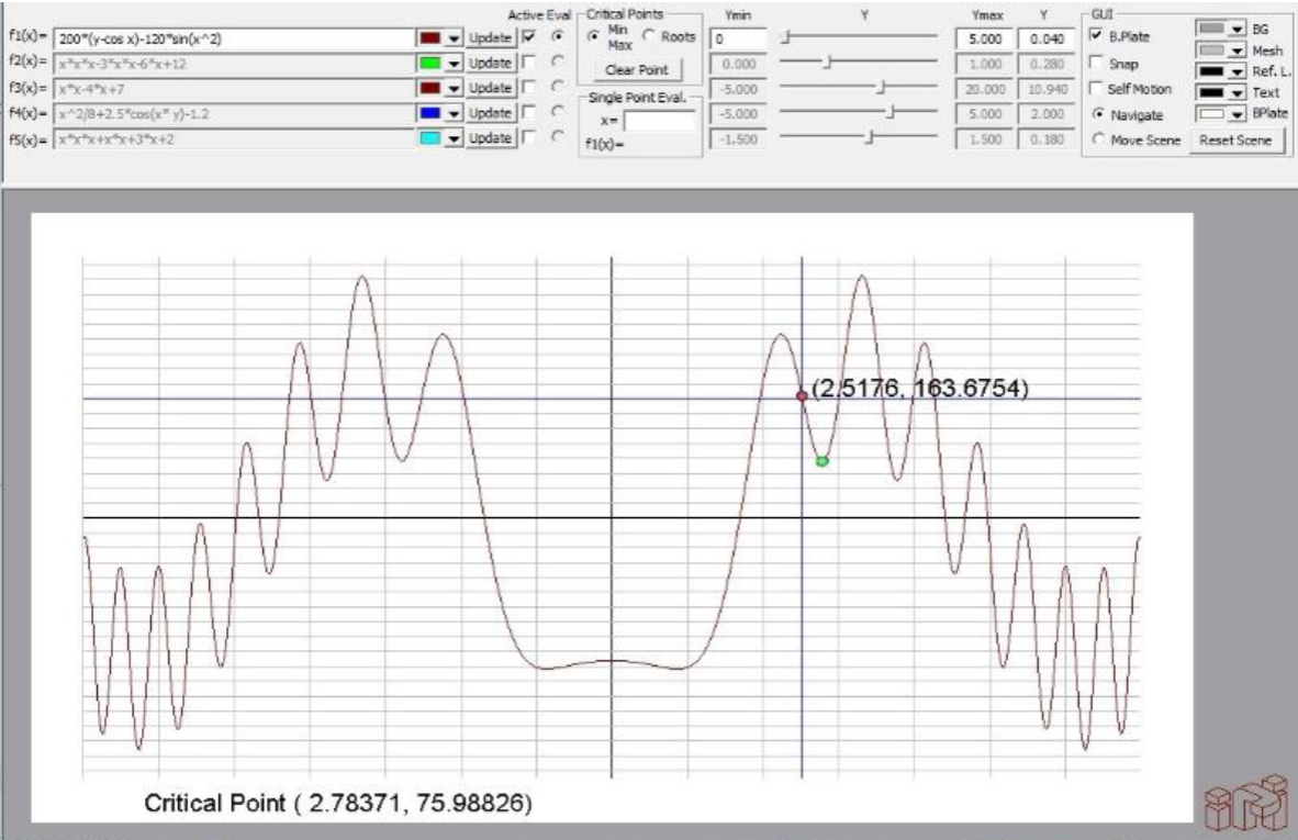
The advantage of having graphical interaction becomes apparent in cases in which there are several minima for a given range, such is the case of the function:

fx,y=200y-cosx-120sinx2 (6)

Equation (6) is plotted in the range (-7, 7) with у = 1/ 25 as shown in Fig. 5. With the motion of the mouse the user can navigate the function and observe its value for any X point; in the snapshot, the mouse is locating a point at (2.5176, 163.6754). At this position if the left button is pressed, the CGoldenSection:: OptimizeO function is called considering that X _s = 2.5176, and, once the line 10 of Fig. 4 is reached, a point is plotted at the closest minimum, and the solution is displayed at the bottom left corner, (2.78371, 75.98826). A similar procedure is followed to find a maximum, but in this case, the right mouse should be pressed.

Fig. 5 Finding a minimum by navigating a function with multiple critical points 

In order to calculate the roots of a function with OptimPloT, one of the following five methods can be chosen: (i) Bisection, (ii) False position, (iii) Fixed Point, (iv) Newton-Raphson and (v) Secant.

4.3 The optimization problem in 3D

The solution of this problem has been widely studied (^{Rao, 2009}), providing various solution methods. The software has implemented the next algorithms, where z≡f( x )=f(x,y)

• ■Powell.

• ■Steepest Descent.

• ■Marquardt.

• ■Davidon-Fletcher-Powell.

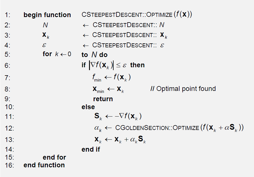
The pseudocode of the steepest descent method is shown in Fig. 6. As in Fig. 4, the iterations allowed, N, and the convergence parameter, ε, are set by default. The initial search vector X ₀ , is gathered from the pointing device; in this case the user can navigate on the surface by moving the mouse. The search direction S _k , is obtained with the aid of the gradient evaluated at x _k . The new searching point is obtained with the aid of the optimal step length α _k , which in turn is obtained with the aid of the function provided in Fig. 4. When the condition of line 6 is satisfied, the solution is stored in (X _min , f _min )

Fig. 6 Pseudocode of Streepest Descent algorithm 

Furthermore, three convergence criteria are established for each of the implemented methods mentioned above. The value of these criteria is compared with a tolerance value, commonly defined by ε. The latter is independent of the convergence criterium, and it is controlled by the user according to the required precision on the solution. Thus, the user can choose the same or different ε value for each criterion for comparison purposes. For example, selecting the same value will provide information on which of the criteria converge faster. The three convergence criteria implemented in OptimPlot are described next:

• ■Grad. Norm.: the norm of the objective function gradient.

• ■Fune. Diffi the absolute difference of the objective function.

• ■Vec. Norm.: the norm of the difference of the solution vector.

As in the case of two-dimension functions, the snapshot shown in Fig. 7, presents a sample with multiple critical points for a three-dimension function. The snapshot indicates the instant the mouse is locating the point (2.7327, 1.9016, -0.0329). In this case the right mouse was pressed and the program converged in four iterations at the closest maximum point (1.5717,3.4015, 4.2594), while popping up the green point, to indicate graphically, which point was reached. Complementary information of this sample is given in Table 2.

Fig 7 Plot of f( x )=ysinx+cos(2y) 

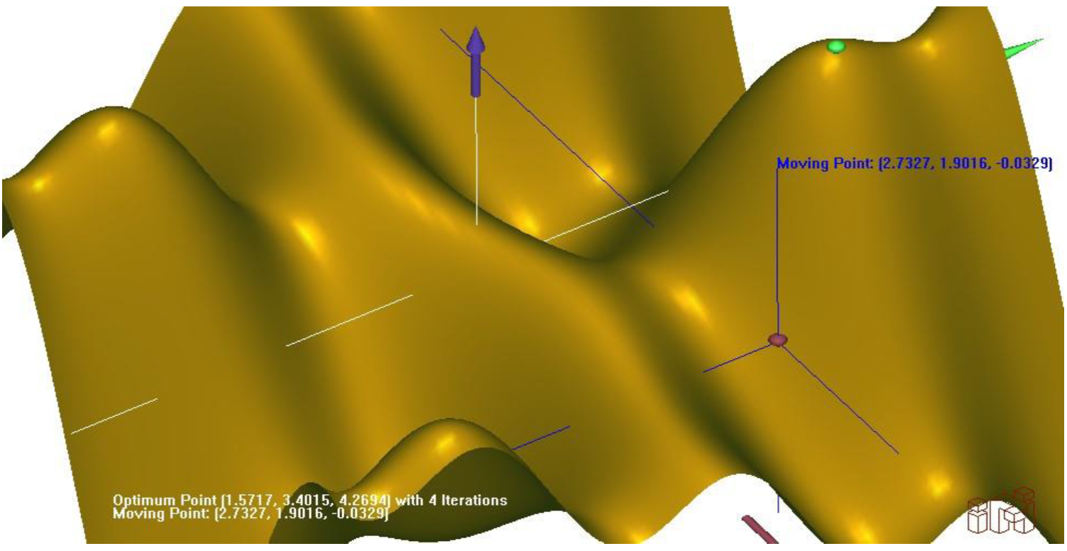
Table 2 Complementary information of Fig.7.  

x range		y range		x0 Red point		xmax Green point		f max
-5	5	-5	5	2.7327	1.9016	1.5717	3.4015	4.2694

5. Examples of analysis

The property of plotting several functions on the same environment extends OptimPlot^´s scope. For instance, with this feature, the user can plot not only the objective function but also the constraints, therefore, the usable-feasible region, can be defined by visual inspection (when the complexity of the problem allows it), or an initial point to start the search can be defined.

5.1 Function analysis on the 2D environment

In order to show the OptimPlot functionality, Fig. 8 shows the plotted responses of a typical second-order control system to a unit step input, thus the underdamped case is given by (Ogata, 2010):

Fig. 8 Unit-step response curves of the second-order control system. 

ft=1-eζωnt1-ζ2sin⁡ωdt+tan-1⁡1-ζ2ζ (7)

where, ζ is the damping ratio (0<ζ<1), ω _η is the undamped natural frequency and ω _η is called the damped

natural frequency,ωd=ωn1-ζ2. From eq. (7), the free parameter is ζ , thus taking ω _η t as the x variable and ζ as y, different cases are plotted by changing the у value.

The first three functions plotted in Fig. 8 represent responses when ζ takes the values 0.03 and 0.6. The fourth function represents the critical damped case, namely, ζ=1. The overdamped case occurs when ζ>1 and is represented by the last function where ζ=2. The correspondent graph for each case can be identified by means of the relating color.

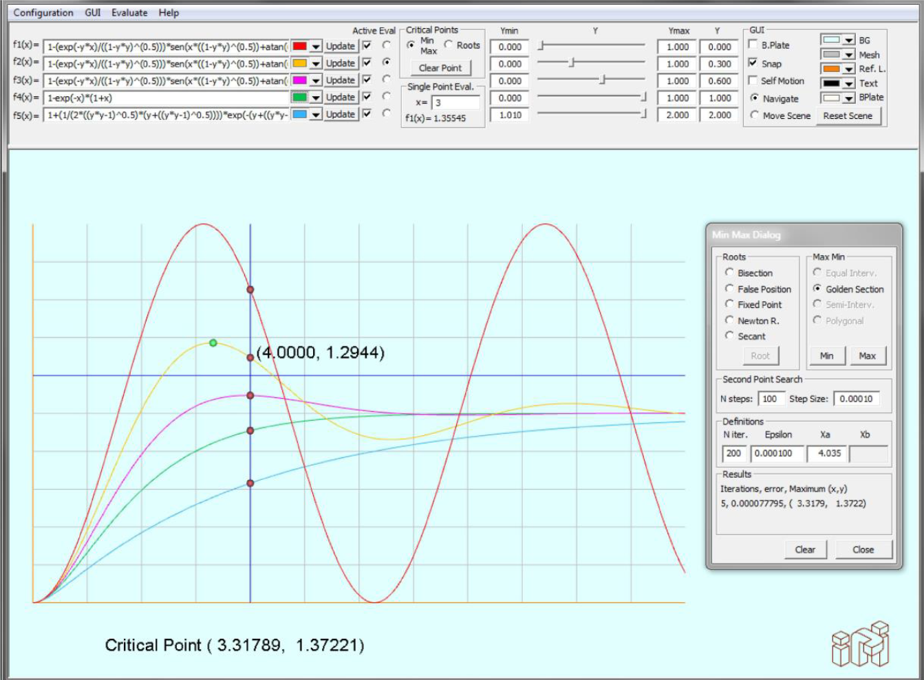
Once the functions are plotted, finding a maximum point is simple. Going back to Fig. 8, a maximum point is found applying the golden section method as the dialog window shows. The critical point that is found is represented by a green point over the function that is selected for evaluation. The access to the dialog window is through the element Evaluate on the menu bar, which opens the Critical Points option, displaying the corresponding dialog window.

The option to find roots is illustrated in Fig. 9, thus, the roots of the function are calculated by a numerical method managed through the Min-Max dialog. In the same figure, the minimum value of the function is shown (in the interval displayed) by means of visual inspection (lower precision).

Fig. 9 The analysis to find function roots in the 2DE. The plotted function is given by X²/8+5/2cos(xy)-6/5 

It is noteworthy to mention that in navigation mode and with the radio button Min-Max active, the user can set the initial point to search for a minimum or a maximum point, by clicking the left button or the right button, respectively, while the cursor is pointing close to the critical point. If the Root radio button is active, the user can search for a root by clicking the left button on each side of the critical point (only in 2DE).

5.2 Function analysis on the 3D environment

The unit-step response curves of a second-order control system can be implicitly plotted in the 3DE. In order to accomplish this task, it is necessary to consider again eq. (7) by taking ω _η t as the x variable and ζ as the у variable (thereby, the ζ variation is visualized in the у direction). The resulting surface plot is shown in Fig. 10. The x axis is identified by the red arrow (bottom-right), in the same manner, the у and Z axis are represented by the green (left) and blue (middle), respectively. To demonstrate the capability of the OptimPlot in the 3DE, the Himmelblau function is plotted, which is shown in Fig. 11. This surface is given by the mathematical expression:

fx=x12+x2-112+x1+x22-72 (8)

Fig. 10 Unit-step response of the second-order control system with wire option in the 3DE. 

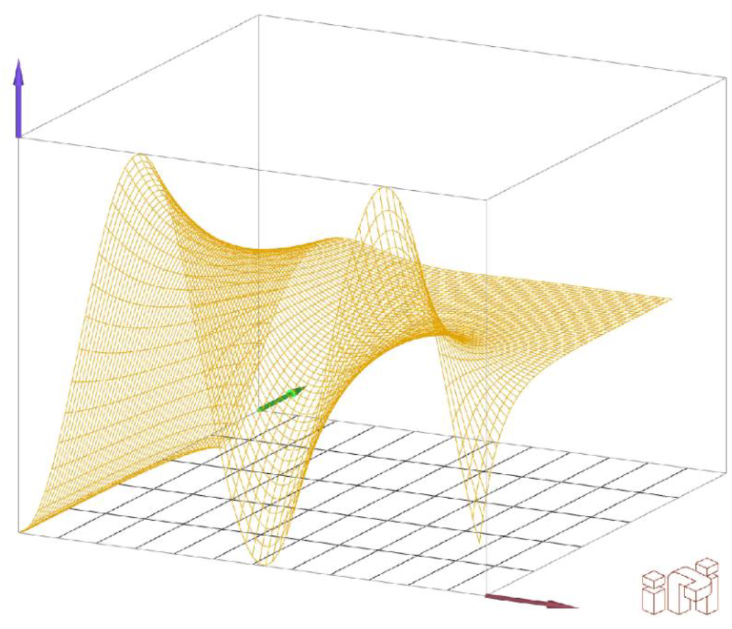
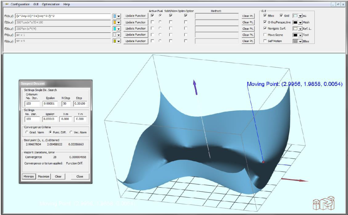
Fig. 11 The steepest descent method application to slve and optimization problem in OptimPlot. The plotted fuction is given by fx=x12+x2-112+x1+x22-72. 

The Himmelblau function has four optimum points, one of them is (3, 2) with ƒ(x*) = 0. To find one of the optimum points, the Steepest Descent method is selected. The dialog window for this method is accessed through the optimization option in the menu bar. To find the minimum, the initial point X ₀ was established (0,0). Moreover, the Fune. Diff. criterion was fixed. The results are shown in Fig. 11, where the dialog window shows the optimal point as (2.99607934,2.00458522) , and the function value evaluated in this point, which is 0.00056663 ; thus, the precision of the solution is determined for the value of the selected convergence parameter, which ins this case was set as ε=1x10^-4 To find an optimum, the use of the numerical method is not always necessary; this can be done by visual inspection if the accuracy is not relevant, as is shown in Fig. 11, where the Moving Point is manually positioned closed to the local minimum.

Because the Himmelblau function has exact optimum points and the corresponding values of f(x*) are integers, it is considered a classical test function in optimization problems. Including the Himmelblau function, in Table 3 are listed five classical test functions (^{Momin & Yang, 2013}); for each function, one optimum point and the corresponding function value are indicated. In Figs. 12 and 13 are shown the optimization results performed in OptimPloT.

Table 3 Test functions and their well-know solution 

Function name	Expression, f(x)	ExactOptimalpoint:x*	f(x´)
Himmelblau	fx=x12+x2-112+x1+x22-72	(3, 2)	0
Goldstein- Price	fx=f1x=f2x, where	(0, ֊1)	3
	f1x=1+x1+x2+1219-14x1+3x12+14x2+6x1x2+3x23
	f2x=30+2x1-3x2218-32x1+12x12+48x2-36x1x2+27x23
Baele	fx=1.5-x1+x1x22+2.25-x1+x1x222+2.625-x1+x1x232	(3, 0.5)	0
Rosenbrock	fx=1-x12+100x2-x122	(1,1)	0
Easom	fx=-cos⁡x1cos⁡x2exp⁡-x1-π2-x2-π	(π, π)	-1

Fig. 12 Goldstein -Price test function and its results with three different algorithms 

Fig. 13 Test functions and their optimum point applying the Steepest descent method 

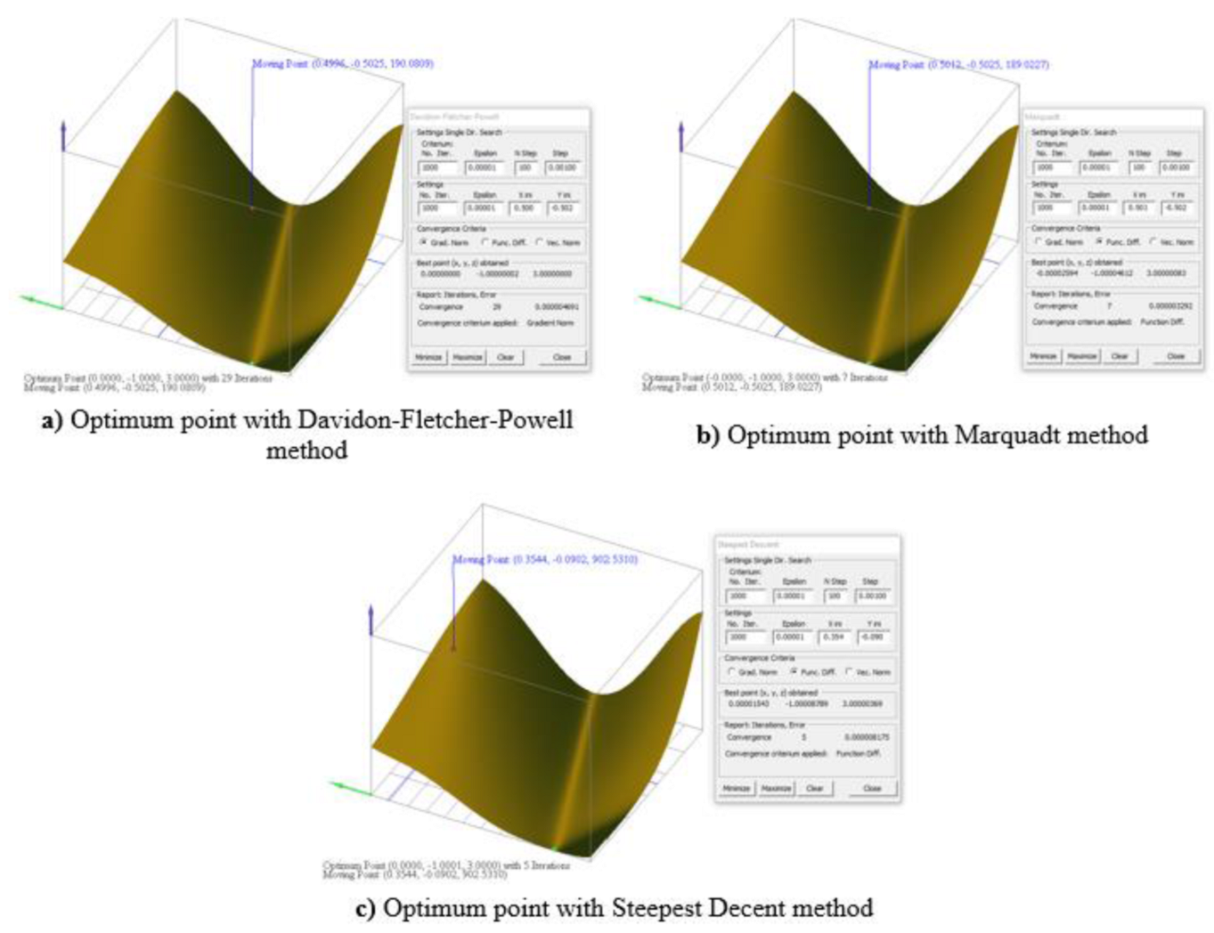
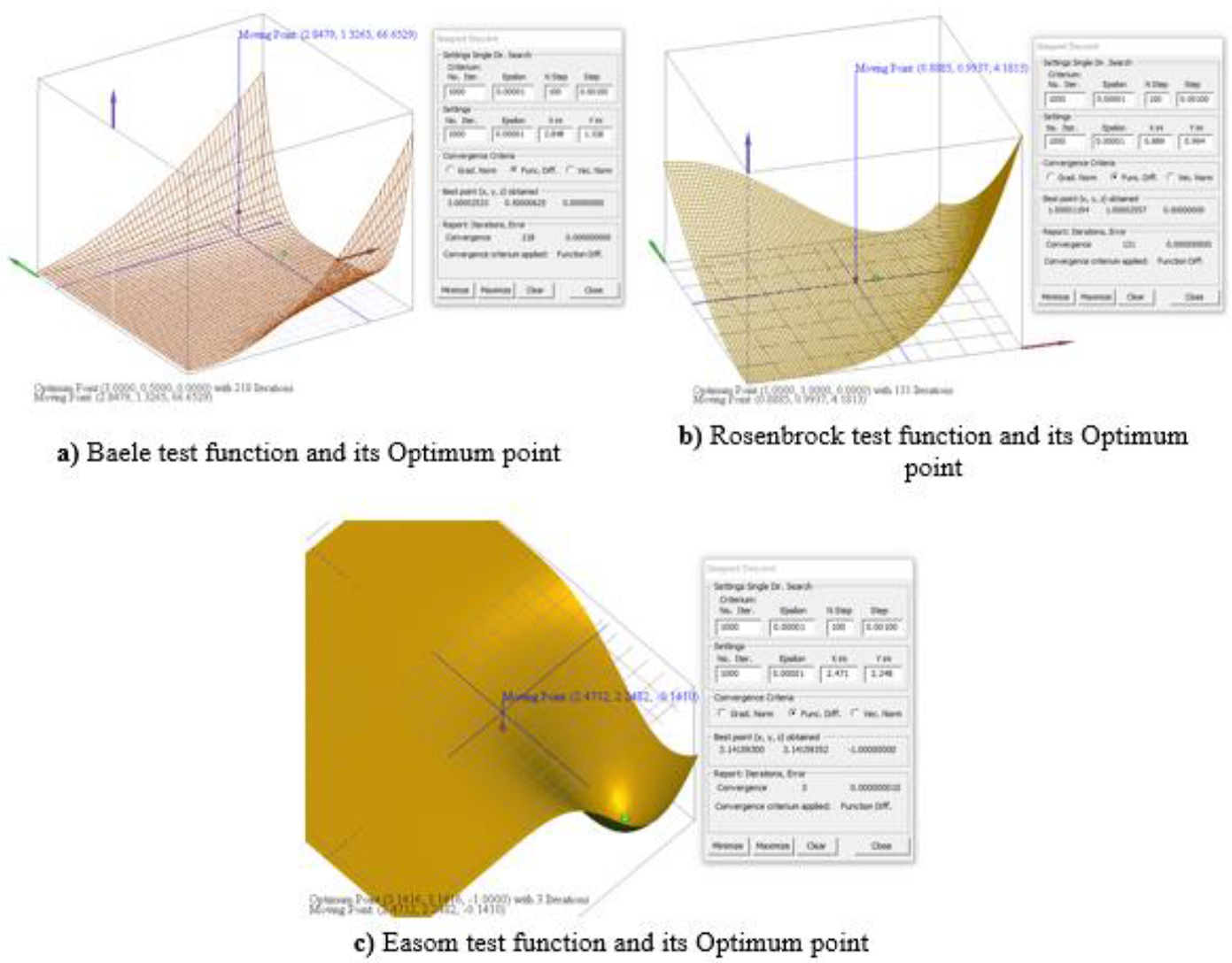
Figure 12 contains three stills of the Goldstein-Price test function solution. In each CetSSţ cl different solution method was applied; the settings to find the optimum point can be observed in the dialog window aside of the graph function, in the same dialog window the user can Report section with the optimum point (Best point) and the function value in this point. Note that the best solution was obtained with the Davidon-Fletcher-Powell method. Moreover, Fig. 13 shows the results of the remaining test functions where the solution was reach applying the Steepest Descent method. In all cases, the initial point X₀, was selected while navigating with the moving point. It is also possible to input X₀ with the aid of the edit boxes X ini and Y ini shown in the dialog box. It is well known that sometimes a given numerical method or a given X₀ , might fail in finding a solution. Thanks to the interactivity of OptimPloT, the user can quickly select a different X₀ or switch for any of the four the optimization methods until the convergence is found. For example, in Fig. 12c, X₀ was initially chosen close to (0.5, -0.5) as in Figs. 12a and 12b, but the report was "no convergence found"; now, with the point (0.354, -0.090), the solution was obtained in five iterations.

Conclusions

This paper is a comprehensive presentation about an optimization software development named OptimPloT. Its structure was explained with the necessary details to show how to create a specific application software on the basis of ADEFID libraries. By using the OOP techniques, it was possible to build a robust and flexible software.

The creation of an interactive software for optimization which releases the user from writing code lines or programming languages was the main aim of this research work. Thus, the user only needs to type the symbolic function expression to see the plotted function, becoming an intuitive handling software. Furthermore, the user can navigate through the function graph to evaluate any point and to establish the initial point to start the search for the optimal value, or the function roots, in the 2DE case.

Some optimization methods were implemented to provide a wide range of options to solve a specific problem. It is possible to include additional optimization methods to improve the software performance.

Several parameters can be changed in-line, in this way the user can immediately observe configuration changes. The full control in the optimization algorithm is another important characteristic, specifically the possibility to set the solution tolerance, setting the convergence criterium to end the algorithm process or fix the maximum iteration numbers.

Finally, once software features have been defined, it is clear that OptimPlot is a software with broad possibilities in education and applied research. Currently, the software is under development, in order to include additional features and solution methods.