


 nova página do texto(beta)
 Inglês (pdf)
 Artigo em XML
 Referências do artigo
 Enviar este artigo por email
 Citado por SciELO
  Similares em
SciELO
Similares em
SciELO 
 Permalink
1. Introduction
A flare system is an essential unit in a petroleum refinery and petrochemical plants. The fuel vapours, while moving upward, entrain air from the surroundings while leaving the tip of the flare stack. The air-fuel mixture is ignited at an appropriate temperature forming a burning flame. Such a flame is known as the diffusion flame. In an alternate arrangement, the fuel is transported in the vapour form through a pipe or burner and is ignited at the tip of the burner. The flame so formed is known as a jet diffusion flame. The degree of turbulence along with flame height and flame geometry depends upon the velocity with which the fuel vapours are released. Understanding the flow and thermal dynamics of a jet diffusion flame is important for the safety of the plant as well as for a number of other scenarios, such as tank leakage or pipeline failure. The intensity of the radiant heat flux from the flame depends on the flame height as well as the height at which the fuel is being released. Hence the determination of the height of a jet diffusion flame is important from the view point of the proper operation of flare system and the plant safety.
The diffusion flames may either be turbulent or laminar, depending on the source Reynolds Number (NRe) (Drysdale, 1985). For NRe < 2100 the flame is considered as a laminar flame, which becomes turbulent as NRe increases to 4000 or more. Laminar diffusion flame has greater height than a turbulent flame. Because of lateral mixing, the turbulent flames have higher reaction/ combustion efficiency; resulting in the consumption of the gas-vapour mixture emanating from the pipe tip at a shorter flame length. The combustion/ reaction in a flame above the pipe tip can be represented as a one-step chemical reaction as follows:
Where, r is the amount of air required to burn 1 kg of fuel vapour, completely. The rate at which the fuel is consumed is given by (Spalding, 1971):
Where, A is a dimensionless pre-exponential factor, p stands for the local pressure (Pa),
The subscripts u and b denote the unburnt and fully burnt conditions, respectively. Obviously, the state of a gas changes from τ = 0 to τ =1 in the course of complete reaction.
The flame length or the flame height (vertical flame) of a jet diffusion flame has been defined in varied ways by various researchers; the axial height from the pipe tip is at which combustion is 99% complete (Hawthrone, Weddell, & Hottel, 1948), the ratio of CO to CO2 is 0.15 (Hottel, 1961), the fuel mole fraction diminished to 0.0005 (Wade & Gore, 1996). The above definitions are based on the concentration of the fuel and have limitations of the accuracy of the concentration measuring device. Newman and Wieczorek (2004) defined the flame length on the basis of the completeness of fuel combustion, relating the yield ratio of CO to CO2. For propane, the yield ratio of CO to CO2 was taken as 0.002. The definition is found to be in agreement with the Heskestad correlation (Heskestad, 1984):
Where, H f is the flame length (m), d is the diameter of nozzle (m). N is a non-dimensional group defined as
Where Q is the heat released from combustion (W) (Heskestad, 1983; Orloff, De Ris, Delichatsios, & Orloff, 1985). c
p
is the specific heat capacity of the reaction mixture (J/kg/K), T
a
is the ambient air temperature (K), ρ
a
is the atmospheric air density at T
a
(kg/m3), r is the stoichiometric air to fuel ratio, d is the burner nozzle diameter (m) and g is the acceleration due to gravity (9.81 m/s2). For most common fuels,
Heskestad (1999) defined the flame length as a function of buoyancy momentum parameter (R M ),
Where, ρ is the density of the reaction mixture (kg/m3). Becker and Liang (1978) correlated the flame height with Richardson number as
and a parameter
Where,
and d is the nozzle diameter (m),
and for cross-wind condition it is given as,
Where, u
*
is the dimensionless fuel velocity and is defined as,
The flame length depends on the extent of reaction/ combustion as also the wind velocity (accounted for by the air entrainment coefficient), gas-vapour velocity, flame temperature, amount of heat radiated out of the flame and flame geometry. It is also affected by fuel properties such as fuel composition, the specific heat and the heat of combustion of the fuel. Gas pressure and frequency of flaring in a flare system also determine the height of flames in flare systems. In a flare system, the source velocity is kept 20% - 30% of Mach number (Ma= u s /v so ), where, v so is the velocity of sound (m/s), for desired flame heights, which in turn determines the amount of heat radiated from the flare.
While flame geometry and source velocity/ stack exit velocity (u s ) is governed by the burner design, flame temperature is a function of u s , wind velocity (v) and the burner design (Leahey, Preston, & Strosher, 2001). For field scale natural gas jet fires, the threshold flame temperature is about 1400 K (Ballie, Caulfield, Cook, & Docherty, 1998). Fairweather, Jones, Lindstedt, and Marquis (1991) used a value of 1200 K for laboratory scale natural gas jet fires. A difference of 200 K in flame temperature will yield a difference of flame length of the order of 20 - 25%. Cumber and Spearpoint (2006) had reported a maximum flame temperature of 1800 K for propane fires by using their probabilistic model. The true flame temperature is less than the adiabatic flame temperature, i.e. T<T d and is limited by large uncertainities. The average radiation temperature also decreases from 1025 oC to 875 oC as wind speeds increased from 1.5 to 3 m/s (Cumber & Spearpoint, 2006). Romero-Jabalquinto, Velasco-Téllez, Zambrano-Robledo, and Bermúdez-Reyes (2016) have presented and described aeronautical use and feasibility of combustion chamber.
In the present paper, an attempt has been made to develop a simplified one-dimensional model to simulate the flame height, flame geometry and temperature. The simulated results for the flame height are also validated with the available experimental data.
2. Mathematical model:
Development of a steady state mathematical model helps in the calculation of the flame height in a stabilized environment. The fire plume formed from a particular fuel is a strong function of the burner design, source velocity and source temperature. The plume once developed, rises due to buoyancy. As the fire plume rises, it entrains air from the surrounding at ambient temperature and thus combustion continues within the reaction zone of the plume. Generally, a fire plume may be divided into two regions, flaming and non-flaming. The flaming region is near the fire source and all combustion takes place in this region. Above this region is the non-flaming zone where practically no reaction takes place. This is characterized as the thermal plume, which contains the non-reactive products (CO, CO2 and water vapours) of combustion along with inert nitrogen and a large amount of ambient air. McCaffrey (1979) further subdivided the flaming region as given below:
This is the region of continuous flame and
In the intermittent region, u is constant and
The mean flame velocity is indistinguishable from the plume velocity in the accelerating region. However, in the intermittent region, sporadic flames are produced, the flame velocity increases until the flame is extinguished, while the mean plume velocity ceases to do so (Gupta, Kumar, & Singh, 1988).
For a flame forming above a cylindrical pipe tip/ orifice, the fundamental conservation equations of mass, momentum and energy can be written as (Bird, Stewart, & Lightfoot, 2002):
Following assumptions can be made for solving the equations of changes under steady state conditions:
Top hat profile governs the radial distribution of temperature and velocity of the flame.
In the laminar jet diffusion flame air is entrained through the exterior surface of the combustion region and the fuel-air mixture is assumed to be convected upward by the fluid flow within the flame zone (Fay, 2006). The entrainment velocity of the surrounding air (v) through the surface of the flame is proportional to the vertical flame velocity (u), i.e.v=αu.
The physical properties of the reaction mixture (fuel + air) remain constant throughout the flaming zone and the pressure along the radial direction of the flaming zone also remains constant.
The fuel enters at ambient temperature and pressure.
Heat is lost only by radiation from the flame surface, having an area of A s .
Using the above assumptions under steady state condition, and integrating the steady state equations across the radius of the flaming region, the following set of ordinary differential equations are obtained:
Where, b is the half plume width and Q r is the radiative heat flux. The reaction rate (-r3) could be expressed in terms of the Arrhenius equation to take into account the effect of temperature on the reaction rate. In such a situation, an equation for material balance of fuel can be written and this could be solved by either finite difference method or shooting method. In order to simplify the model, the heat generation term by combustion reaction is expressed as follows (Drysdale, 1985):
Where,
The total amount of heat radiated per unit area (Q r ) is expressed according to Stefan-Boltzman’s relation.
Where, the emissivity (ε) is equal to 1, for hydrocarbons (Drysdale, 1985).
Equations (17), (18), (19) and the constitutive relationships, (20)-(21), along with the boundary conditions complete the mathematical description of the jet diffusion flame. The following boundary conditions can be used:
The boundary conditions, Equation (22), refer to the characteristics of the fire source/ burner at any time (t), after the commencement of fire. Initially, it can be assumed that T s =T a , where T a is the ambient temperature. The Equations (17), (18), (19) can be written in the following explicit forms:
Equation (24) includes the terms of heat generation by reaction and heat loss by radiation in addition to the entrainment term. Fire is considered as a reaction phenomenon, where the fuel from its liquid or solid state gets converted to its gaseous form prior to the onset of combustion. The density of this gaseous reaction mixture (kg/m3) changes with temperature of the fire plume following the ideal gas law:
Where, P is the ambient pressure (Pa), M is the molecular weight of the reaction mixture (kg/mol), R is the universal gas constant and T is the flame temperature (K). The subscript ‘a’ denotes the air/ ambient condition.
As the fuel gases move upward, air from the surroundings gets entrained according to the equation v=αu. All the air entrained by the fuel gases does not get mixed with the fuel instantaneously, and a significant mass of entrained air does not participate in the combustion/ reaction. Thus, only a represents of the mass fraction of the entrained air (φ) is actually taking part in combustion, on mixing with the fuel, at a particular location of entrainment. This parameter, φ is a function of the fuel velocity (u). Hence, the mass burning rate of the fuel in Equation (24) is estimated according to the following relation:
Here, φ is the reaction mixing efficiency parameter,
Equations (23), (24) and (25) can be solved numerically by using fourth order Runge-Kutta method, with a step size of 0.01, using the boundary conditions and the Equations (26) and (27) for various values of Froude number. The flame height can be defined as the axial distance from the tip of the burner to the top at which the mass flow rate of the reaction mixture becomes zero, i.e.
This means, the flame height is the axial distance at the end of which the fuel combustion is complete and combustible mixture ceases to exist.
3. Results and discussions:
The developed set of model Equations (23) through (25) along with the boundary conditions (Equation 22) and Equations (26) and (27) has been simulated numerically with the help of fourth order Runge - Kutta method. This method is applicable for both linear and non-linear ordinary differential equations. The method possesses an error of the order of ∆z5 per step and an accumulated error of the order of ∆z4, where ∆z is the step size. A value of 0.01 is taken as the step size. A source code has been developed in MATLAB, version 7.0.1.24704 to solve the model equations. The processing time required is 15 s. The input parameters of Zukoski, Kubota, and Cetegen (1981) have been used for the solution of the model equations.
Zukoski et al. (1981) had carried out experiments in the laboratory to determine the height of the jet diffusion flame above burners of different sizes. The fuel used in the experiment was a mixture of hydrocarbons. The fuel contained mainly of methane (0.924 mole fraction), ethane (0.042 mole fraction), nitrogen (0.015 mole fraction) and propane (0.01 mole fraction). The specific heat capacity of the fuel is taken as 2150 J/kg/K, according to its composition. The lower heating value (heat of combustion) of the fuel is taken to be 47.5 MJ/kg and its density is taken to be 0.72 kg/m3. The flame produced is assumed to be axisymmetric; and for such a flame, air entrainment coefficient varies from 0.1 to 0.15. The values of the initial source velocity and the burner sizes are given in Table 1.
Table 1 Input Parameters (Zukoski et al. 1981).
| Burner Diameter (m) | Initial Source Velocity (m/s) | Air Entrainment Coefficient (α) |
|---|---|---|
| 0.1 | 0.588 | 0.11 |
| 0.1 | 2.355 | 0.11 |
| 0.1 | 3.532 | 0.11 |
| 0.2 | 0.416 | 0.11 |
| 0.2 | 0.866 | 0.11 |
| 0.2 | 1.248 | 0.11 |
Physical properties of air, viz. molecular weight of air, and density of air are taken from literature (Perry, Green, & Maloney, 1984). The stoichiometric coefficient is calculated from the fuel parameter (Heskestad, 1999), as described in Section-3, and found to be 15.323. The initial fuel source temperature is taken as 300 K, which is the same as the ambient temperature.
3.1 Flame heights:
Table 2 gives a comparison of flame heights as calculated by using the empirical/ semi-theoretical equations proposed by different researchers, for various values of Froude number
Table 2 Comparison of the Calculated Values of Flame Height from Different Models.
| bs | Fr | Calculated Values of Flame Height (m) Using the Equations of | |||||
|---|---|---|---|---|---|---|---|
| Heskestad (1984) | Hustad & Sonju | Cook et. al. | MITI Model | Considine & Grint | Sion-Tan (1967) | ||
| 0.05 | 0.594 | 1.995 | 1.773 | 0.996 | 1.889 | 0.525 | 12 |
| 0.05 | 2.377 | 3.55 | 2.339 | 1.932 | 3.29 | 1.05 | 12 |
| 0.05 | 3.566 | 4.193 | 2.537 | 2.346 | 3.869 | 1.286 | 12 |
| 0.1 | 0.297 | 2.975 | 3.087 | 1.637 | 2.863 | 0.883 | 24 |
| 0.1 | 0.618 | 4.057 | 3.574 | 2.325 | 3.839 | 1.274 | 24 |
| 0.1 | 0.891 | 4.729 | 3.845 | 2.768 | 4.444 | 1.529 | 24 |
Table 3 shows the comparison of the values of the calculated flame height by the present model with the experimental data of Zukoski et al. (1981). The predictions by Cook et al. (Frank & Lees, 1996) and Considine and Grint (Frank & Lees, 1996) are also used for the purpose of comparison. The results of the one dimensional model developed in the present work are in complete agreement with the experimental data of Zukoski et al. (1981). The flame height calculation by the present model assumes that the combustion takes place with some fraction of the entrained air at the elevation of entrainment. From Table 3 one can see that, as the Froude number (Fr) increases the flame height also increases for each of the burner type. This is because of poor mixing of fuel and air in the reaction zone. The predictions from this one dimensional model, however, do not take into account effect of wind vector on the radiative heat flux from the flame, which would affect the flame height depending on the prevailing wind velocity, as reported by Sengupta, Gupta, and Mishra (2011) and Da Silva and Landesmann (2014). Both these work employs the point source model (providing larger heat flux) to determine the diffusion pool fire flame height under the various wind conditions. We are in the process of developing more realistic mathematical model that would take the wind velocity effect on the jet diffusion flame height.
Table 3 Comparison of Estimated Flame Heights (m) with Zukoski et al. (1981), Experimental Data, and other Jet Flame Models.
| b s | Fr | Zukoski et al. (1981), (Expt. data) | Cook et al. | Considine & Grint | Present Model | Deviation (%) | |
|---|---|---|---|---|---|---|---|
| Cook et al. | Considine & Grint | ||||||
| 0.05 | 0.594 | 1 | 0.996 | 0.525 | 1 | 0.4 | 47.5 |
| 0.05 | 2.377 | 1.5 | 1.932 | 1.05 | 1.5 | -28.8 | 30.0 |
| 0.05 | 3.566 | 2.3 | 2.346 | 1.286 | 2.3 | -2.0 | 44.1 |
| 0.1 | 0.297 | 1 | 1.637 | 0.883 | 1 | -63.7 | 11.7 |
| 0.1 | 0.618 | 1.5 | 2.325 | 1.274 | 1.5 | -55.0 | 15.1 |
| 0.1 | 0.891 | 2.3 | 2.768 | 1.529 | 2.3 | -20.4 | 33.5 |
Figure 1a illustrates the variation of H f /d with Fr, where d is the diameter of the burner and is equal to 2b s . For a given burner diameter increase in Fr increases the H f /d ratio, and hence forming a jet flame. This is because an increase in the source velocity increases the mass flow rate of the fuel, which results in greater flame heights. Moreover, narrower burner produces jet flames of higher H f /d ratio for a fixed Fr. The logarithmic plot between H f /d ratio and Fr (Figure 1b) shows that H f /d varies linearly with Fr, with a slope of 0.6 (hydrocarbon mixture flame (Thomas, 1962) for all burner diameters.
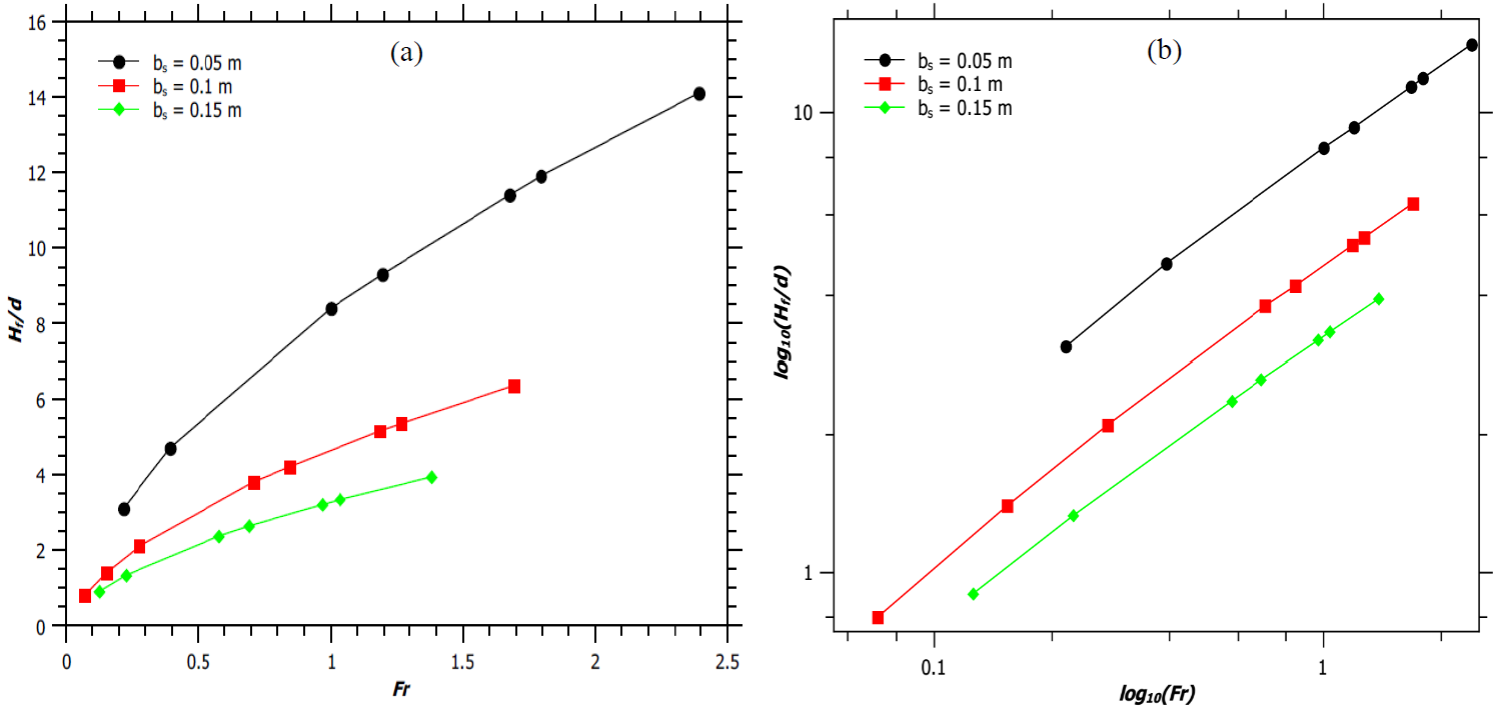
Fig. 1 (a) Variation of H f /d ratio with Froude number. (b) Logarithmic plot of H f /d ratio with Froude number.
An increment in source velocity amplifies the H f /d ratio, as shown in Figure 2. A jet flame with greater H f /d ratio is found to have a higher value of Q * (Figure 2), where
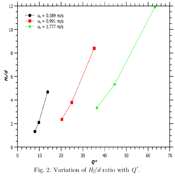
Zárate, Lara, Cordero, and Kozanoglu (2014) have also reported of an initial increase in the total heat flux with an increase in the flame height of a jet flame.
3.2 Flame temperature and reaction mixing efficiency parameter:
Figure 3, gives the axial temperature profile within the flame, for different Fr. With an increase in Fr, the height of attaining the maximum flame temperature (T max ) also increases. This is because of the fact that the mass burning rate increases with an increase in the stack exit velocity. A decrease in reaction mixing efficiency parameter (φ) at Fr = 3.566 and 0.891 (Figure 3a) further increases this height for attainment of T max . It has been observed that, the temperature of the flame increases initially because of combustion; as it is an exothermic process. The total heat loss due to radiation is not significant at this stage. In the later stage as the flame rises upwards, the heat loss due to radiation increases as the flame temperature rises. Because of the radiation loss, the flame temperature starts decreasing particularly along the flame height at the end of the combustion zone. Secondly, in the combustion zone; fuel combustion generates heat energy that causes an increase in temperature of the reaction mixture close to the adiabatic flame temperature as the radiant heat loss is less significant in this part of the flaming region. At the upper edge of the combustion region, however, most of the fuel has been consumed and there is no further increase in the thermal energy, though an increase in the momentum flux in this region (refer Figure 8a) increases the air entrainment, which along with predominant radiant heat loss cools the reaction mixture. This phenomenon results in the formation of a peak in the temperature distribution, as shown in Figure 3a. A similar trend of the temperature profile was also observed by Cumber and Spearpoint (2006) from their mathematical model of propane jet flame. Wang, Li, Mei, and Mi (2013) also noted similar temperature profile along the flame height, for different volume fraction of oxygen taking part in the combustion.
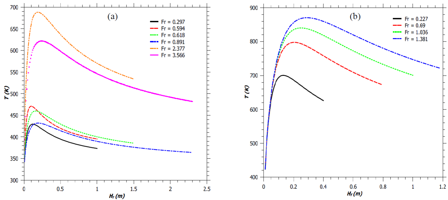
Fig. 3 Axial flame temperature of a jet flame. (a) Flames described by Zukoski et al. (1981). (b) Simulated flames.
From the experiment of Zukoski et al. (1981) and also from the present model (illustrated in Figure 3a), it is observed that, for the burner with b s = 0.05 m; an initial increase of source velocity (u s ) from 0.588 m/s to 2.355 m/s (75% increase) results in a 33% increase in flame height (H f ). Further increase in source velocity, for the same burner, by only 33% increases H f by 35%. Similarly, for the burner with b s = 0.1 m; an initial increase in u s by 52%, followed by an increase of 31% increases the flame height by 33% and 35%, respectively. While the initial 33% increase in H f is because of the enhancement in mass flow rate of the fuel alone, the increase of H f by 35% later, with a relatively small increment in u s (as against of 75% and 52%, respectively) is due to the combined effect of the increase in the mass flow rate of the fuel and a decrease in the reaction mixing efficiency parameter (φ). The reduction in the mixing time of the fuel with air with an increase in the Fr to 3.566 and 0.891, for the burners with diameters of 0.1 m and 0.2 m, cause a decrease in the value of φ (Figure 4a) and hence reduces the T max by 6.5% and 11% (Figure 3a), respectively. For the burner diameter of 0.5 m we also observe an initial increase in the value of φ followed by a decrease with an increase in the Fr (Figure 4a). Thus, for all the experimentally generated flames as reported in the literature from each of the three burner designs (Zukoski et al., 1981); the present model shows a decrease in the value of φ following an increase in its value with an increase in the Fr (Figure 4a). However, for a given amount of mixing between the fuel and the entrained air; T max increases with an increase in Fr for a given burner dimension (Figure 3b). This is because of the increase in the mass burning rate of the fuel with an increase in u s . The reduction in the value of φ with an increase in the flare stack exit velocity is found to follow the following inequality, for all the cases studied by the present model:
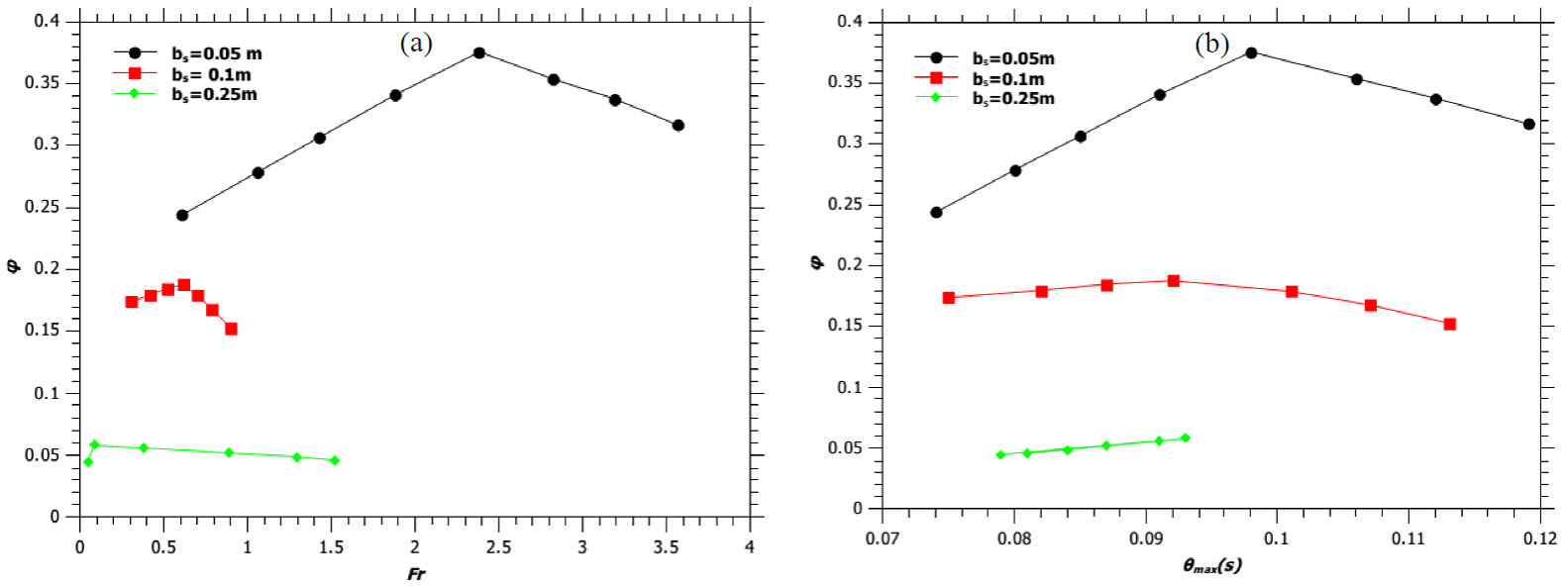
Fig. 4 (a) Variation of reaction mixing efficiency parameter (φ) with Froude number. (b) Variation of reaction mixing efficiency parameter (φ) with θmax. Solid lines are guide way to eyes.
Where, b max is the maximum half plume width attained by the jet flame and u max is the maximum velocity of the fuel at the top of the flaming region. Thus, θ max in some way gives the measure of the time required by the flame to attain its fully developed geometry. Figure 4b shows the variation of reaction mixing efficiency parameter (φ) with θ max for burners with diameter 0.1m, 0.2 m and 0.5 m and we observe that the reaction mixing efficiency parameter decreases for all values of θ max > 0.1.
Figure 5a shows the variation of T max with source velocity, u s . For a given value of φ, an increase in the flow rate of the fuel from the burner of fixed diameter increases the mass burning rate and hence the maximum temperature of the flame. Similarly, the T max is found to be greater for a flame with greater flame height (H f ) and with fixed reaction mixing efficiency parameter of 40%, as shown in Figure 5b. Similar trends of T max with u s and H f were reported by Cumber and Spearpoint (2006). Moreover, it is noted from Figures 5a and 5b that a decrease in burner diameter reduces the maximum flame temperature and enhances the flame height. Thus, it can be concluded that, as the flame become more jet-like (greater H f /d ratio) with b s decreasing; the maximum flame temperature decreases, while the maximum flame temperature increases with increasing flame height due to an increase in stack exit velocity.
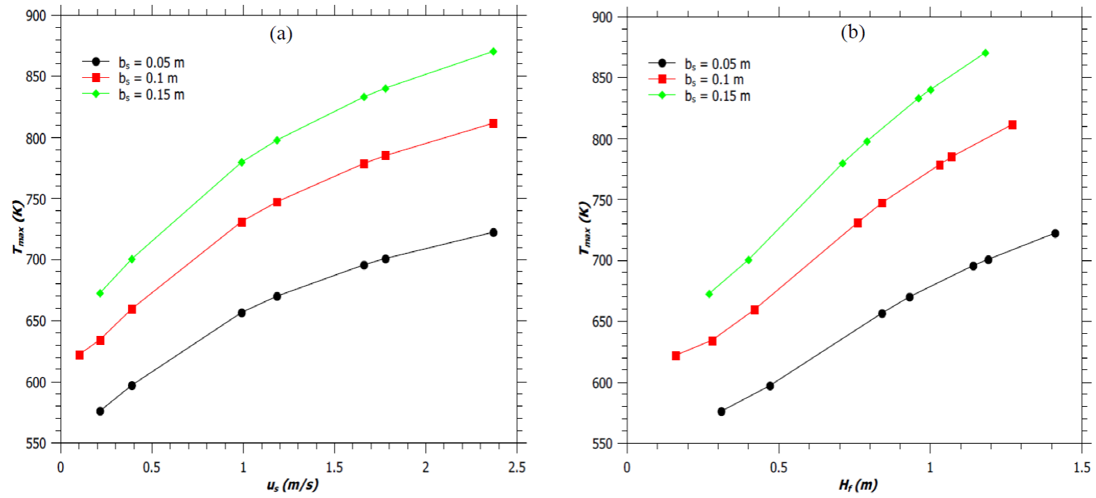
Fig. 5 (a) Variation of maximum flame temperature (T max ) with source velocity (u s ). (b) Variation of maximum flame temperature (T max ) with flame height (H f ). Solid lines are guide way to eyes.
Moreover, it is noted from Figures 5a and 5b that a decrease in burner diameter reduces the maximum flame temperature and enhances the flame height. Thus, it can be concluded that, as the flame become more jet-like (greater H f /d ratio) with b s decreasing; the maximum flame temperature decreases, while the maximum flame temperature increases with increasing flame height due to an increase in stack exit velocity.
3.3. Flame geometry and velocity:
The velocity profile within the flame and the flame geometry has been obtained using the present model for the flames described by Zukoski et al. (1981). Figure 6 shows the flame geometry for various Fr values. The flame geometries for jet diffusion flames as reported by Zukoski et al. (1981) et al. (1981) and for jet diffusion flames with fixed reaction mixing efficiency and for fixed burner design have been illustrated in Figure 6a and Figure 6b, respectively. For Fr < 1.0, the flame width initially decreases along the flame height. This phenomenon is known as the ‘necking of the flame’. At this point, the half width of the plume is minimum, b min .
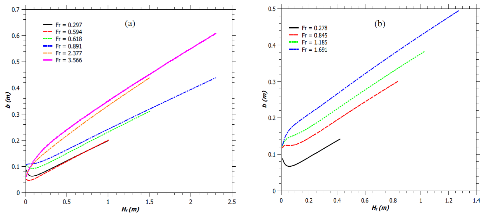
Fig. 6 Radius of the flaming zone in a jet flame. (a) Flames described by Zukoski et al. (1981). (b) Simulated flames.
Thereafter, b starts increasing and the flame assumes the shape as described by Gupta (1990) and also by the Carven model (Frank & Lees, 1996). The b min is about 0.046 - 0.092 m for all the low values of Fr. Figure 7 shows the variation of the maximum radius, b max , of the flaming zone with Froude number. It’s seen that for any given b s value, the b max increases with an increase in Fr. Similarly, for any Fr value, b max increases with an increase in b s . As the fuel-air mixture rises, the vertical jet velocity increases as shown in Figure 8. This results in an increase in the entrainment of air into the plume according to the equation, v=αu, as discussed earlier. The increasing air entrainment increases the volume of the reaction mixture and results in an increase of the flame width (Figure 7). Moreover, for a fixed Fr, burner with narrower diameter produces flame of smaller width, as shown in Figure 7. Hence jet flame with higher H f /d ratio, have smaller flame width, as expected (by comparing Figures 1a and 7).
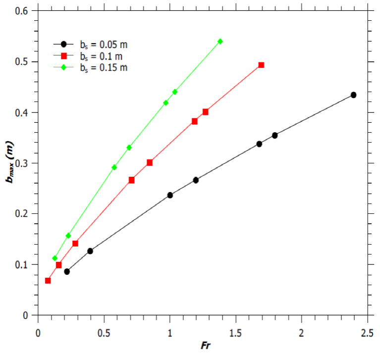
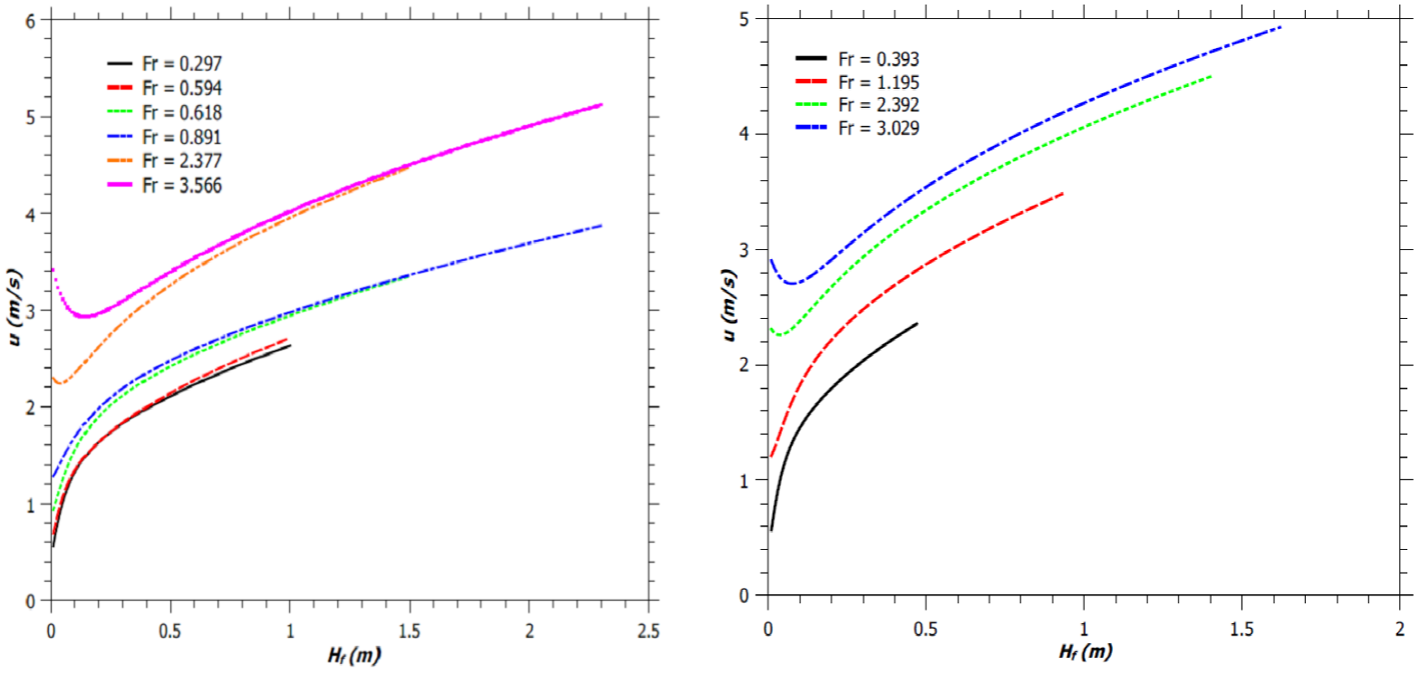
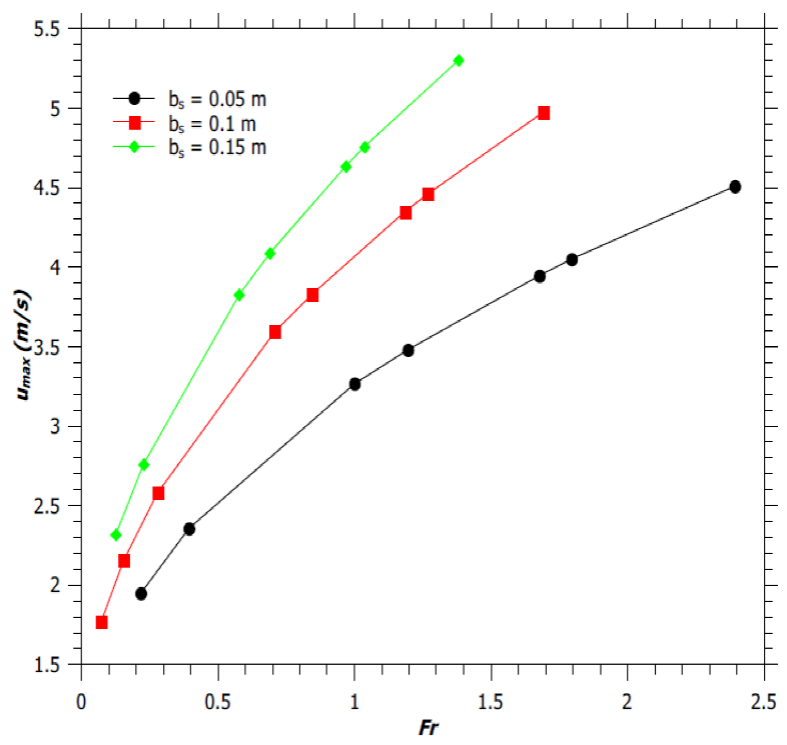
Fig. 8 Vertical jet flame velocity. (a) Flames described by Zukoski et al. (1981). (b) Simulated flames.
The variations of the axial flame velocity for jet diffusion flames as reported by Zukoski et al. (1981) and for jet diffusion flames with fixed reaction mixing efficiency and for fixed burner design have been illustrated in Figure 8a and Figure 8b, respectively. From Figure 8, we can observe that the vertical flame velocity increases until the flame gets extinguished. This was reported by McCaffrey (1979) too. For Fr < 2.0, the vertical flame velocity increases monotonically with the flame height. This result in more entrainment of air and hence an increase in the flame width. For Fr > 2.0, there is an initial decrease of flame velocity followed by its monotonic increase along the flame height. An increase in Fr increases the maximum flame velocity, due to enhanced inertia and buoyant force. However, for a fixed Fr, a burner with a narrower diameter produces a flame with lower vertical flame velocity, as shown in Figure 9. Thus, jet flame with higher H f /d ratio, has lower maximum vertical flame velocity at the tip of the flaming region, as expected (by comparing Figures 1a and 9).
4. Conclusion:
The one dimensional jet diffusion flame model in a flare system can be used to predict the behavior of the flare - the axial temperature profile, the flame geometry, and its velocity variation along the flame length. The developed one-dimensional model provides correct estimate of the experimentally determined flame height under no wind conditions, though we obtain a narrower peak in the temperature distribution along the flame height as compared to the data reported in literature (Cumber & Spearpoint, 2006). The flame height to burner diameter (H f /d) ratio, as predicted by the model, is found to approach a value of jet-like flames with an increase in the stack exit velocity and with a decrease in the burner diameter. However, the logarithmic variation of this ratio with the Froude number is linear having a constant slope of 0.6.
Due to an increase in temperature within the flame, vertical flame velocity increases because of increased buoyancy until the end of the flaming region of the plume. The plume rises mainly due to the buoyant force. A minimum initial fuel source velocity is required for the jet flame to form. The total quantity of the fuel is not combusted with the amount of immediately entrained air. This phenomenon is illustrated with a reaction mixing efficiency parameter (φ). The fraction of the fuel-air mixture reacting in the flame depends on the reaction time available for the fuel-air mixture. The fraction of air thus taking part in the reaction is determined by the value of φ. It is observed that, φ, initially increases with an increase in stack exit velocity (u s ); because of more entrainment of air; and thereafter decreases as the reaction time available decreases with an increase in u s . The in-crease in the value of φ is limited by the value of θ max , which is to be less than 0.1 s to maintain the increase in the reaction mixing efficiency parameter with the change in u s .
The width of the jet flame produced by a flare system increases after an initial necking over a short flame length, for Fr < 1.0. The necking of the flame decreases with an increase in stack exit velocity. The height of the flame mainly depends on the initial mass flow rate of the fuel and also on the extent of combustion of fuel-air mixture, taking place in each grid. While the heat generation is by the combustion/ reaction, the heat loss takes place mainly due to radiation. As a consequence of the process of combustion and radiation occurring simultaneously, a jet diffusion flame which is formed with higher H f /d ratio has smaller flame width and lower maximum vertical flame velocity at the tip of the flame.
The prediction of the flame geometry by the present one dimensional jet diffusion flame model corresponds to the flame geometry predicted by Gupta (1990) and by the Carven model (Frank & Lees, 1996). The predicted flame height of the jet diffusion flame is in good agreement with the experimentally observed flame height, given by Zukoski et al. (1981). However, it is clearly seen that the flame height as calculated from the various models available in literature give results that varies widely as compared to the experimentally observed flame height.

