


 nueva página del texto (beta)
 Inglés (pdf)
 Artículo en XML
 Referencias del artículo
 Enviar artículo por email
 Citado por SciELO
  Similares en
SciELO
Similares en
SciELO 
 Permalink
1. Introduction
In all process industries measurements of level, temperature, pressure and flow parameters are very vital. Real time systems provide many challenging control problems due to their dynamic behavior, uncertainty and time varying parameters, constraints on manipulated variables, dead time on input and measurements, interaction between manipulated and controlled variables and unmeasured frequent disturbances. Because of the inherent non-linearity, most of the chemical process industries are in need of modern control techniques. Nonlinear systems like conical tanks find wide applications in gas plants and petrochemical industries. They are preferred because of the advantages like better disposal of solids, easy mixing and complete drainage of solvents such as viscous liquids in industries. In conical tank non-linearity exists due to its variation in cross-sectional area. Because of the non-linearity, level control is a challenging task in conical tank and its demands for implementation in real time. The nonlinearities also exists due to the saturation-type introduced by maximum or minimum allowed level in tanks, valve geometry, flow dynamics, pumps and valves. The most basic and pervasive control algorithm used in the feedback control is the proportional, integral and derivative (PID) control algorithm. PID control is a widely used control strategy to control most of the industrial automation processes because of its remarkable efficiency, simplicity of implementation and broad applicability. The long history of its practical use and proficient working dynamics are some of the pivotal reasons behind the large acceptance of the PID control. A PID controller attempts to correct the error between a measured process variable and a desired set point by calculating and then providing a corrective action that can adjust the process accordingly. In this paper, the modeling of the system, calibration of various transmitters associated with the conical tank system, tuning of PID parameters for the level control of a conical tank setup is considered. The open loop test is performed to obtain process reaction curve and mathematical model of the process. Based on the mathematical model, gain tuning of the PID controller is done using the Cohen Coon tuning method which is implemented in the real time system to get optimum settling time and rise time. Fuzzy control, an intelligent control method imitating the logical thinking of human and being independent on an accurate mathematical model of the controlled object, can overcome some shortcomings of the traditional PID. The controller designed using fuzzy logic implements human reasoning that has been programmed into fuzzy logic language (membership functions, rules and the rules interpretation). Fuzzy logic is a form of many values logic which deals with reasoning that is approximate rather than fixed and exact. Compared to traditional binary sets (where variables may take on true or false values), fuzzy logic variables may have a truth value that ranges in degree between 0 and 1. Fuzzy logic has been extended to handle the concept of partial truth, where the truth values may range between completely true and completely false. Fuzzy logic has been applied to many fields from control theory to artificial intelligence. Fuzzy logic has rapidly become one of the most successful technologies for developing sophisticated control systems. It is interesting to note that the success of fuzzy logic control is largely due to the awareness to its many industrial applications. But the fuzzy algorithm cannot adapt for large range of working environments. So Kalman algorithm is used.
Some related researches study this problem of tuning PID controllers. Models enable predictions about how a process will change when perturbed or modified. Many different approaches have been proposed for using local models to approximate non-linear systems.
Ahn and Truong (2009) presented a novel online method using a robust extended Kalman filter to optimize a Mamdani fuzzy PID controller. The robust extended Kalman filter (REKF) is used to adjust the controller parameters automatically during the operation process of any system applying the controller to minimize the control error.
Alleyne, Lui, and Wright (1998) presented a new kind of hydraulic load simulator for conducting performance and stability tests for control forces of hydraulic hybrid systems. In the dynamic loading process, disturbance makes the control performance (such as stability, frequency response, loading sensitivity, etc.) decrease or turn bad. In order to improve the control performance of a loading system and to eliminate or reduce the disturbance, an online self-tuning fuzzy proportional-integral-derivative (PID) controller is designed.
Sakthivel, Anandhi, and Natarajan (2011) designed a real time fuzzy logic controller based on Mamdani type model for controlling the liquid level in a spherical tank. Since the process is non-linear, the model is designed at three different operating regions (at level 30 cm, 45 cm, and 60 cm). The process model is experimentally determined from step response analysis and is interfaced to spherical tank in real time using VAMT-01 module through MATLAB.
Cheng, Zhong, Li, and Xu (1996) designed a high-accuracy and high-resolution fuzzy controller to stabilize a double-inverted pendulum at an upright position successfully. A new idea of dealing with multivariate systems is described.
Fukami, Mizumoto, and Tanaka (1980) proposed a method which involves an inference rule and a conditional proposition which contains fuzzy concepts. And also pointed out that the consequence inferred by their methods does not always fit our intuitions and suggested the improved methods which fit our intuitions under several criteria.
Garcia-Benitez, Yurkovich, and Passino (1993) proposed a two level hierarchical control strategy to achieve an accurate endpoint position of a planar two-link flexible manipulator. The upper level consists of a feedforward rule-based supervisory controller that incorporates fuzzy logic, whereas the lower level consists of conventional controllers that combine shaft position-endpoint acceleration feedback for disturbance rejection properties and shaping of the (joint) actuator inputs to minimize the energy transferred to the flexible modes during commanded movements.
Guo, Zhou, and Cui (2004) introduced a hybrid fuzzy control system of the furnace. Applied the fuzzy control strategy to short period prediction of the furnace temperature and Combining fuzzy control with PID control, the heavy oil flux is achieved by using the online self-adjusting capability of the harmonious factor. And the self-optimization fuzzy control of the ratio of air to fuel becomes realized.
Jwo and Wang (2007) used the traditional approach for selecting the softening factors heavily relies on personal experience or computer simulation. In order to resolve this shortcoming, a novel scheme called the adaptive fuzzy strong tracking Kalman filter (AFSTKF) is carried out.
Kobayashi, Cheok, and Watanabe (1995) described a fuzzy rule-based Kalman filtering technique which employs an additional accelerometer to complement the wheel-based speed sensor, and produce an accurate estimation of the true speed of a vehicle. The Kalman filters are used to deal with the noise and uncertainties in the speed and acceleration models, and fuzzy logic to tune the covariances and reset the initialization of the filter according to slip conditions detected and measurement-estimation condition.
Kwon (2006) suggested a robust Kalman filtering method of adopting a perturbation estimation process which is to reconstruct total uncertainty with respect to the nominal state equation of a physical system. The predictor and corrector of the discrete Kalman filter are reformulated with the perturbation estimator. In succession, the state and perturbation estimation error dynamics and the covariance propagation equations are derived. In the sequel, the recursive algorithm of combined discrete Kalman filter and perturbation estimator is obtained. The proposed robust Kalman filter has the property of integrating innovations and the adaptive capability of the time-varying uncertainties. An example of application to a mobile robot is shown to validate the performance of the proposed scheme.
Wang and Yuan (2012) developed a self-tuning fuzzy PID control method of grate cooler pressure based on Kalman filter to overcome the frequent varying working condition and worse signal-to-noise radio of pressure signals. Based on dynamic simulation and characteristics analysis of the clinker cooling system, the system variables were determined, then the control model of grate cooler was obtained by system identification.
Gaeid (2013), designed an appropriate Kalman filter (KF) with optimal gain as well as the two degree of freedom compensator for the DC motor and verified the stability of the proposed algorithm and the noise sensitivity.
Muniandy, Samin, and Jamaluddin (2015) explains how the derivative kick problem arises due to the nature of the PID controller as well as the conventional fuzzy PID controller in association with an AARB. The authors proposed two types of controllers: self-tuning fuzzy proportional-integral-proportional-derivative (STF PI-PD) and PI-PD-type fuzzy controller.
The Kalman filter provides an effective means of estimating the state of a system from noisy measurements, given that the system parameters are completely specified. The innovations sequence for a properly specified Kalman filter will be a zero-mean white noise process. However, when the system parameters change with time, the Kalman filter has to be adapted to compensate for the changes. Traditionally, this has been accomplished by using nonlinear filtering, parallel Kalman filtering and covariance matching techniques. These methods have produced good results at the expense of large amounts of computational time. An adaptive algorithm which employs fuzzy logic rules is used to adapt the Kalman filter to accommodate changes in the system parameters. The adaptive algorithm examines the innovations sequence and makes the appropriate changes in the Kalman filter model.
2. Conical tank setup
The real time system consists of one input (inflow) and one output (level of the tank). The inflow is taken from a reservoir tank through a centrifugal pump with single phase motor. The inlet pipe has a Rota meter, Electromagnetic type flow meter called as flow transmitter (FT1), air-to-open type pneumatic control valve (CV) and a hand valve to monitor and control the flow rate. The outlet has a hand valve, Electromagnetic type flow meter called as flow transmitter (FT2) and air-to-open type pneumatic CV. The tank level is measured using a DPT, called as level transmitter (LT). The level in the tank is directly proportional to the pressure created by liquid in it. LT measures the level by measuring pressure at bottom of the tank with reference to the atmosphere and coverts into an electrical quantity (4-20 mA). The LT is energized with 24 V DC source and lower range value (LRV) and upper range value (URV) are set using a highway addressable remote transducer (HART) communicator. The layout of the conical tank setup is shown in Fig. 1.
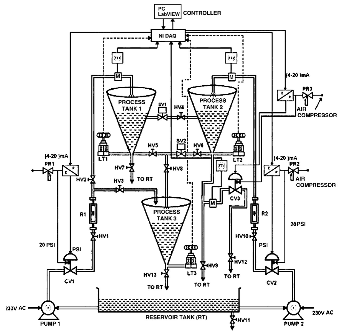
The system is interfaced to the computer through NI USB 6211 data acquisition card (NI DAQ) and it can handle a maximum of 10 V, so the DPT outputs (4-20 mA) are converted into 2-10 V using a 500 resistances and scaled up using LabView. The controller signals (0-10 V) from computer via NI DAQ are converted into 4-20 mA using a voltage to current convertor and given to current to pressure (E/P) convertor. The pneumatic line from the compressor is connected to an air regulator and its output is given as constant inputs (20 psi) for two different E/P converters. The CVs are operated based on the pneumatic outputs from E/Ps.
3. Estimation of transfer function and PID gain
3.1. Transfer function for the system
The open loop response is plotted and the values obtained from the plot like percentage change in level (Q %), delay time (t d), the time taken by the level are used for getting mathematical model of the conical tank. The model of first order process is as in Eq. (1). The first order process with time delay (FOPTD) model is,
Time constant τ = 960 s.
Eq. (2) indicated above is the obtained mathematical model for the entire operating range of the conical tank system.
4. Fuzzy controller
Fuzzy control has been widely used in industrial controls, particularly in situations where conventional control design techniques have been difficult to apply. Number of fuzzy rules is very important for real time fuzzy control applications. This paper proposes a novel approach called block based fuzzy controllers. This study is motivated by the increasing need in the industry to design highly reliable, efficient and low complexity controllers.
The proposed block based fuzzy controller is constructed by several fuzzy controllers with less fuzzy rules to carry out control tasks. The fuzzy logic controller involves four main stages: Fuzzification, rule base, inference mechanism and defuzzification. For the systems where the physical modeling is difficult and information regarding the model is inadequate for applying any control action, Fuzzy logic actions are applied over it. Fuzzy logic systems are based on logical reasoning along with ability to fuzzify any system which helps in easy implementation. In many industrial processes, fuzzy logic controllers are used due to which takes the control action like human and the controlling process is simple once it is designed. Mainly FLC are implemented on non-linear systems which yield for better results. For designing the controller number of parameters needs to be selected and then Membership Function and rules are selected based on heuristic knowledge. There are two inputs to the fuzzy controllers: absolute error |e(t)| and absolute derivative of error |de(t)|. The ranges of these inputs are from 0 to 1, which are obtained from the absolute values of system error and its derivative through scale factors chosen from the specification of the nonlinear system. For each input variable, triangle membership functions (MFs) are requested to use.
In practice, fuzzy control is applied using local inferences. That means each rule is inferred, and the results of the inferences of individual rules are then aggregated. The most common inference methods are: the max-min method, the max-product method and the sum-product method, where the aggregation operator is denoted by either max or sum, and the fuzzy implication operator is denoted by either min or prod. Fig. 2 shows the basic fuzzy structure. Especially the max-min calculus of fuzzy relations offers a computationally nice and expressive setting for constraint propagation. Finally, a defuzzification method is needed to obtain a crisp output from the aggregated fuzzy result.
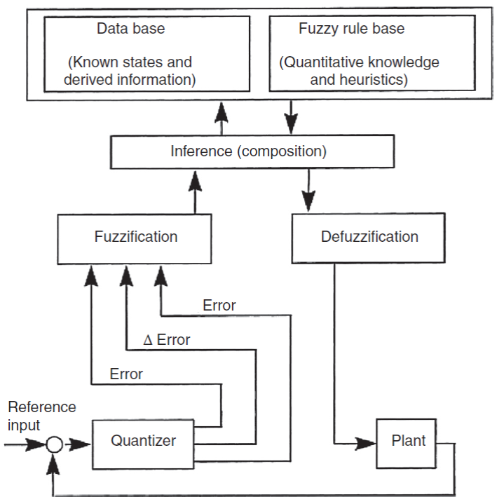
Popular defuzzification methods include maximum matching and centroid defuzzification. The centroid defuzzification is widely used for fuzzy control problems where a crisp output is needed, and maximum matching is often used for pattern matching problems where we need to know the output class. Hence, in this study, the fuzzy reasoning results of outputs are gained from aggregation operation of fuzzy sets of inputs and designed fuzzy rules, where max-min aggregation method and centroid defuzzification method are used.
4.1. FIS editor
Two inputs are defined for the fuzzy controller. One is the level of the liquid in the tank denoted as “level” and the other one is the rate of change of liquid level in the tank denoted as “rate”. Both of these inputs are applied to the rule editor. According to the rules written in the rule Editor the controller takes the action and governs the opening of the valve which is the output of the controller and is denoted by “valve”. The FIS editor is shown in Fig. 3.

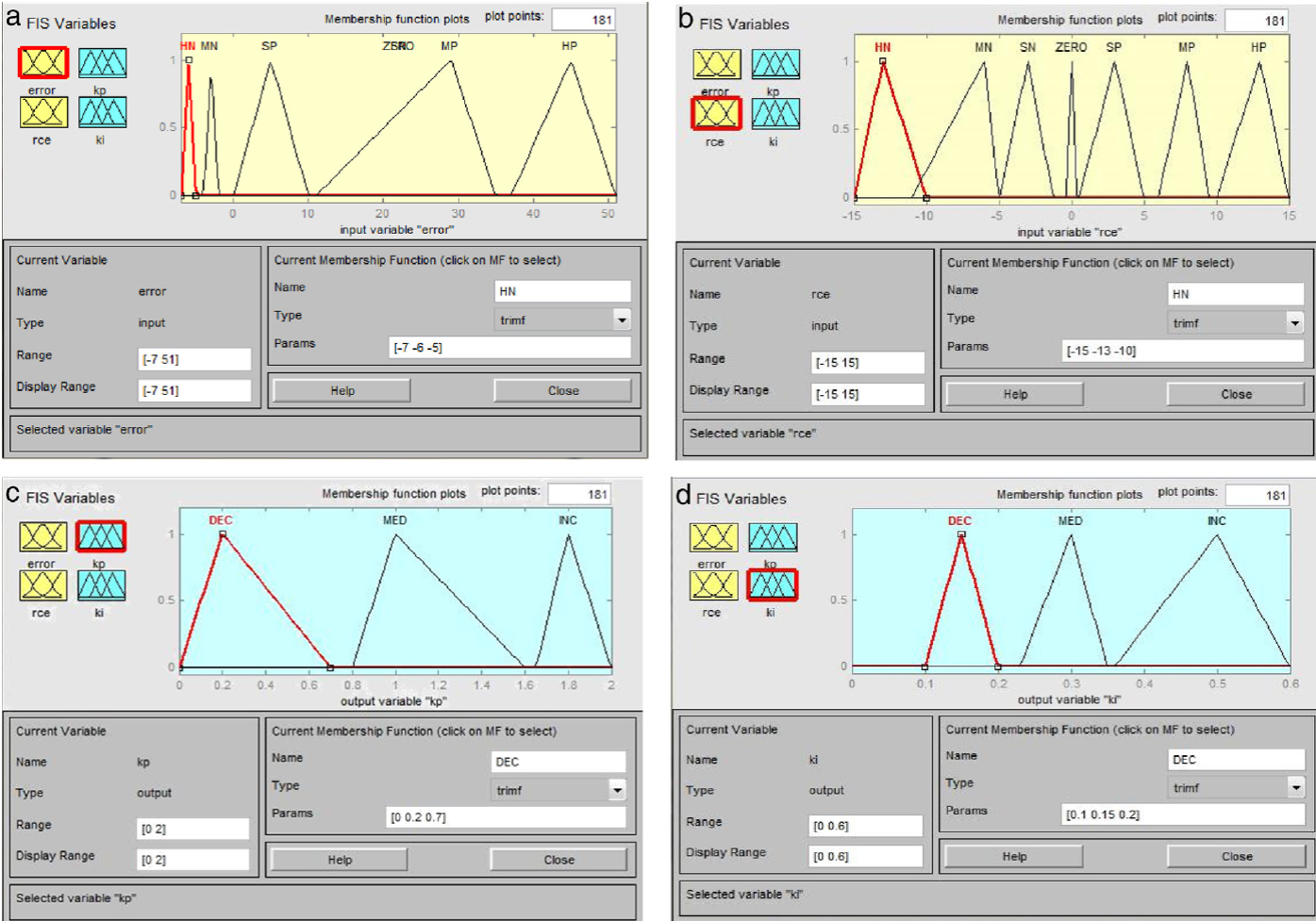
4.2. Membership function editor
The membership function editor shares some features with the FIS editor. In fact, all of the five basic GUI tools have similar menu options, status lines and help and close buttons. The membership editor shown in Fig. 4 is the tool that lets you display and edits all of the membership functions associated with all of the input and output variables for the entire fuzzy inference system. When you open the membership function editor to work on a fuzzy inference system that does not already exist in the workspace, there are not yet any membership functions associated with the variables that you have just defined by the FIS editor. The membership editing is done for every input and output variables. For the first input variable named error, the range for the input variable is from −7 to +51. The membership editing for the second input variable named rce ranges from −15 to +15. Similarly the membership editing carried out for the first output variable ranges from 0 to 2 for the first output variable named K p. The second output variable named K i range is from 0 to 0.6. For the level control of conical tank process, input and output membership functions are designed as shown in Fig. 4 and both inputs and outputs consist of seven functions. The out-put variables from FLC K p and K i will be used to tune the PID controller for better performance.
4.3. Rule viewer
The rule viewer allows you to interpret the entire fuzzy inference process at once. The rule viewer also shows how the shape of certain membership functions influences the overall result. Since it plots every part of every rule, it can become unwieldy for particularly large systems, but for a relatively small number of inputs and outputs it performs well (depending on how much screen space you devote to it) with up to 49 rules. The rule viewer shows one calculation at a time and in great detail. In this sense, it presents a sort of micro view of the fuzzy inference system. To observe the entire output surface of the system and the entire span of the output set, based on the entire span of the input set, by open up the surface viewer. The rules formed are shown in Table 1.
Table 1 Rule table.
| Error | RCE | ||||||
|---|---|---|---|---|---|---|---|
| HN | MN | SN | ZERO | SP | MP | HP | |
| HN | K p = dec | K p = dec | K p = dec | K p = dec | K p = dec | K p = dec | K p = dec |
| K i = dec | K i = med | K i = inc | K i = dec | K i = inc | K i = med | K i = dec | |
| MN | K p = med | K p = med | K p = med | K p = dec | K p = dec | K p = dec | K p = dec |
| K i = med | K i = med | K i = inc | K i = inc | K i = inc | K i = inc | K i = inc | |
| SN | K p = dec | K p = dec | K p = dec | K p = dec | K p = dec | K p = dec | K p = dec |
| K i = dec | K i = med | K i = inc | K i = med | K i = inc | K i = med | K i = inc | |
| ZERO | K p = med | K p = med | K p = med | K p = med | K p = med | K p = med | K p = med |
| K i = dec | K i = med | K i = inc | K i = med | K i = inc | K i = med | K i = med | |
| SP | K p = dec | K p = inc | K p = med | K p = med | K p = med | K p = med | K p = dec |
| K i = dec | K i = inc | K i = med | K i = med | K i = med | K i = med | K i = dec | |
| MP | K p = med | K p = inc | K p = inc | K p = inc | K p = inc | K p = med | K p = inc |
| K i = dec | K i = inc | K i = inc | K i = dec | K i = inc | K i = med | K i = med | |
| HP | K p = inc | K p = inc | K p = inc | K p = med | K p = inc | K p = inc | K p = inc |
| K i = dec | K i = med | K i = inc | K i = med | K i = med | K i = med | K i = inc | |
inc, increase; dec, decrease; med, medium.
Obtained FLC simulation results are plotted against with that of conventional controller PID controller for comparison purposes. The simulation results are obtained using a 49 rule FLC. Rules shown in the rule editor provide the control strategy. Here these rules are implemented in the above control system. For comparison purposes, simulation plots include a conventional PID controller and the fuzzy algorithm. As expected, FLC provides good performance in terms of oscillations and overshoot in the absence of a prediction mechanism. The FLC algorithm adapts quickly to longer time delays and provides a stable response while the PID controllers, drives the system unstable due to mismatch error generated by the inaccurate time delay parameter used in the plant model. From the simulations in the presence of unknown or possibly varying time delay, the proposed FLC shows a significant improvement in maintaining performance and preserving stability over standard PID method. To strictly limit the overshoot using Fuzzy control can achieve greater control effect. Fig. 5 shows the rule viewer.

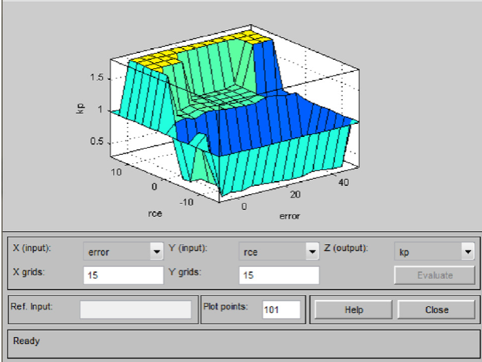
In this paper, liquid level is taken and MATLAB is used to design a fuzzy control. Then we analyze the control effect and compare it with PID control. Especially it can give more attention to various parameters such as the time of response, the error of steadying and overshoot. Comparison of the control results from these two systems indicated that the fuzzy logic controller significantly reduced steady state error. The surface viewer is shown in Fig. 6
5. The Kalman algorithm
The need for accurate state estimates often arises in control systems applications. The performance of a state estimator is usually judged by two criteria. First, the estimator needs to be accurate. Therefore, the mean error should be as small as possible, ideally zero. The estimator also needs to provide a precise estimate of the current state. Therefore, the covariance of the error should be small. The optimal estimate based on the error variance criterion is called the minimum variance estimate. The Kalman filter provides an effective means of solving the minimum variance estimation problem for a linear system with noisy measurements linearly related to the states. A linear discrete system can be described by the following set of equations.
System model
where w(k) is a zero mean white process noise with covariance Rw.
Measurement model
where v(k) is a zero mean white process noise with covariance Rv.
The Kalman filter algorithm can be viewed as a predictor corrector algorithm as shown in Fig. 7.
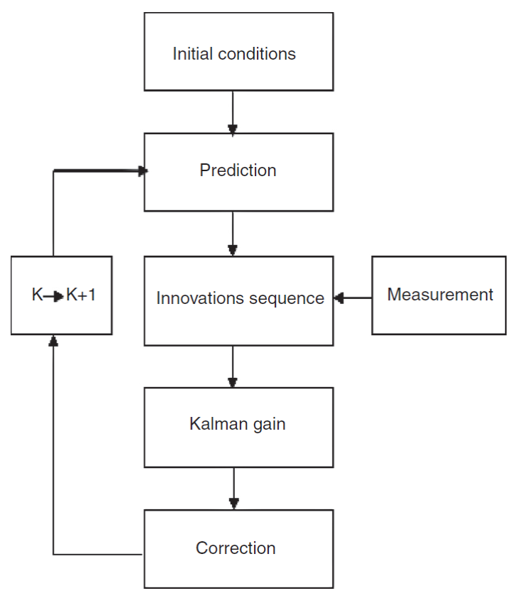
The Kalman filter algorithm shown in Fig. 7 assumes that the system state transition matrix, measurement model and the covariance’s of the plant and measurement noise are known. This is rarely the case in the real world. A properly specified Kalman filter will have the properties given in Table 2. Adaptive filtering is an online process of trying to identify unknown system parameters based on the measurements and innovations sequence as they occur in real time. The innovations sequence of a properly specified Kalman filter should be a purely random process. Several techniques have been suggested for dealing with filtering problems when the system contains unknown parameters. Nonlinear filtering has been successfully applied to the problem of system identification (i.e. state transition matrix and/or measurement model contain unknowns).
Table 2 Properties of properly specified Kalman filter.
| 1 | Innovations sequence is zero-mean. |
| 2 | Innovations sequence is white. |
| 3 | Innovations sequence is un correlated in time. |
| 4 | Innovations sequence lies within the confidence interval constructed from R e of the Kalman filter algorithm. The innovations sequence will have a normal distribution. Therefore, less than five percent of the innovations will be outside two estimated standard deviations. The confidence interval is then constructed using the following equations. |
| Upper limit = 2.0 sqrt (R e ) | |
| Lower limit = −2.0 sqrt (R e ) | |
| 5 | The actual variance of the innovations sequence will be reasonably close to the estimated variance, R e . |
| 6 | The error estimation lies within the confidence limits constructed from the estimated error covariance, |
| Upper limit = 2.0 sqrt( |
|
| Lower limit = −2.0 sqrt( |
|
| 7 | The actual error variance is close to the estimated variance. |
As shown in Fig. 8, the proposed method uses the standard Kalman filter equations and adapts the system parameters based on the innovations sequence. The fuzzy logic adaptive algorithm examines the innovations sequence and determines what type of change in model parameters is necessary to insure that the sequence is a zero mean white process. A certain amount of a priori information about the system is necessary in constructing the control rules for adapting the filter parameters.

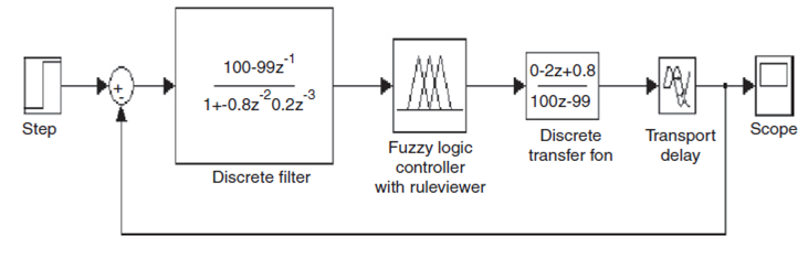
6. Simulink model of fuzzy and PID controller
Simulink is a Matlab toolbox designed for the dynamic simulation of linear and nonlinear systems as well as continuous and discretetime systems. It can also display information graphically. Matlab is an interactive package for numerical analysis, matrix computation, control system design, and linear system analysis and design available on most CAEN platforms (Macintosh, PCs, Sun, and Hewlett-Packard). In addition to the standard functions provided by Matlab, there exist a large set of toolboxes, or collections of functions and procedures, available as part of the Matlab package. Fig. 9 shows the Simulink model for fuzzy and PID controller.

7. Simulink model of fuzzy with Kalman algorithm
The Simulink model of the Kalman algorithm along with fuzzy controller and plant is as shown in Fig. 10.
8. Results and discussion
The response obtained from the plant model by using FLC and PID controller is as shown in Fig. 11. From the response, it can be clearly seen that the response obtained from the fuzzy controller is more accurate and precise when compared to conventional controller. Parameters like response time, peak overshoot, settling time are fast, less and accurate compared to PID controller.
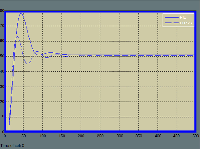
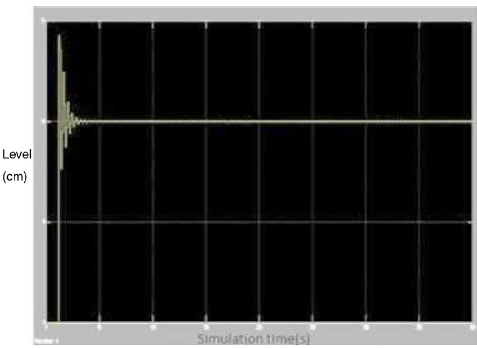
In this research work, the liquid level is taken and MATLAB is used to design a fuzzy control. Then we analyze the control effect and compare it with PID control. Especially it can give more attention to various parameters such as the time of response, the error of steadying and overshoot. Comparison of the control results from these two systems indicated that the fuzzy logic controller significantly reduced steady state error. Even though the response of the fuzziness is more accurate and precise than PID, the plant is still sensible to external noise. In order to remove that noise and make the system change its parameters accordingly, Kalman algorithm is used here. Kalman algorithm is used because of its ability to provide the quality of the estimate and itsrelatively low complexity. The result obtained by using Kalmanfilter is as shown in Fig. 12.
Figs. 13 and 14 show the front panel and block diagram panel of a LabView simulator of a level estimator. The fuzzy model is developed using Matlab simulink. On the Simulink Model toolbar, NORMAL simulation is changed as EXTERNAL simulation. The simulation configuration parameters are changed. Then the model is built. In LabView new VI is built with the desired indicators and controls. The simulink model and Labview VI are saved in same location. In SIT Connection manager the correct Simulink parameter is selected that goes along with the LABVIEW LABEL and TYPE. Then the NI DAQ and mappings are configured. This is where the input and output channels are selected. Select an input or output from DAQ CHANNELS that is being used. Select the corresponding Simulink input/output from MODEL INPUTS/OUTPUTS. When both boxes contain a highlighted item, select ADD. This will map the input/output. Make sure that all desired indicators are present. Connect a wire from the SIGNALS input of the block to the wire that goes into the desired indicator. Now the program can be executed.
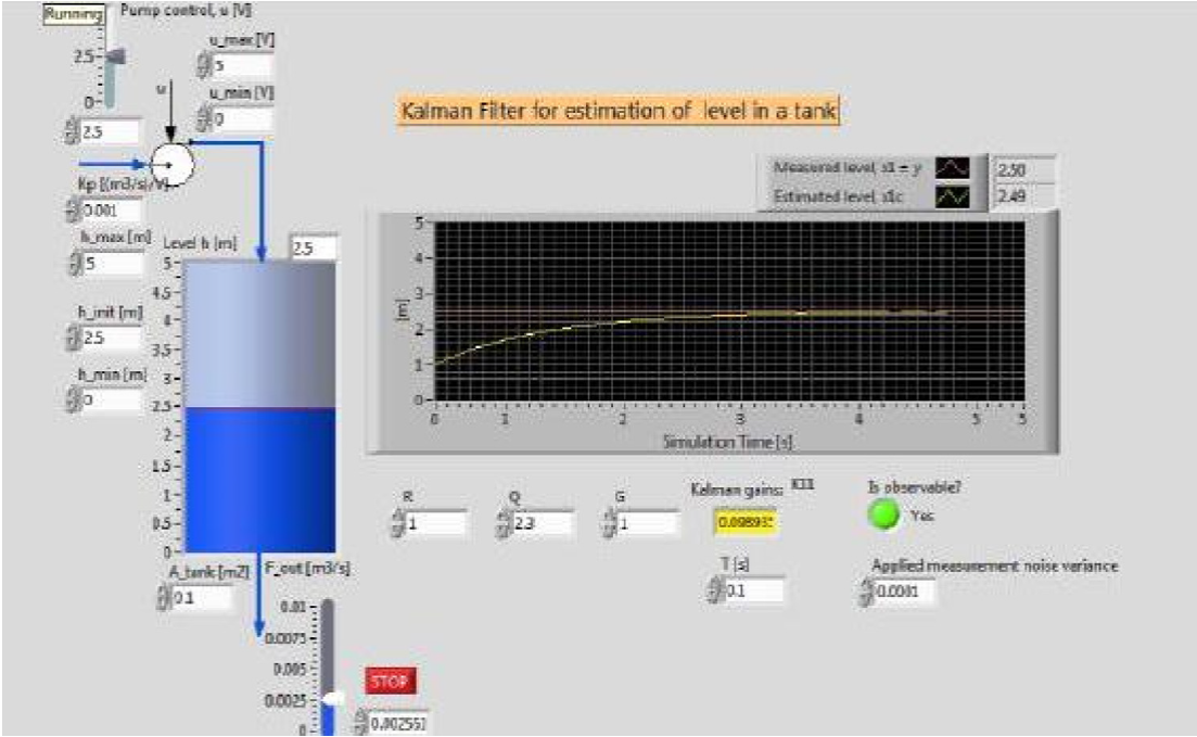
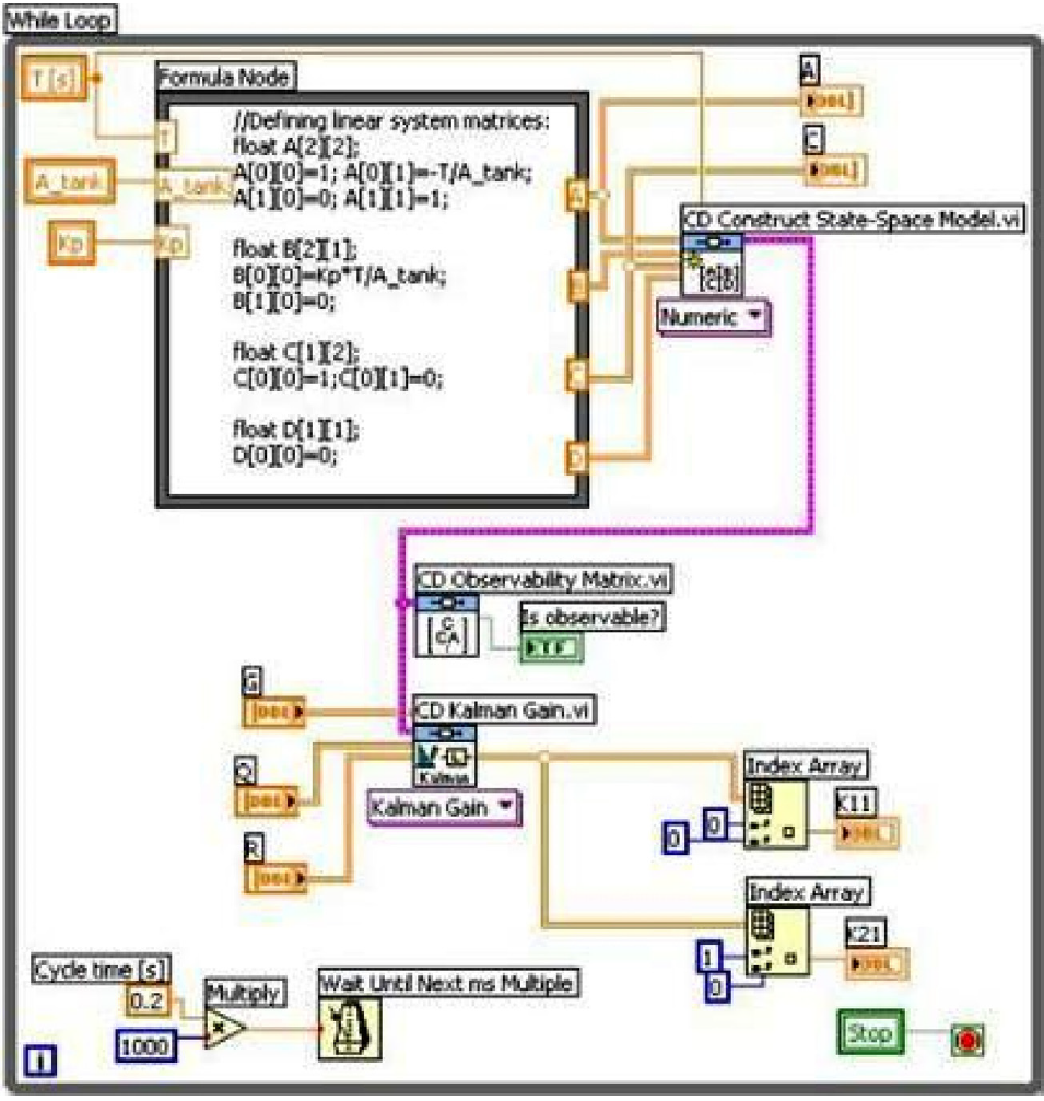
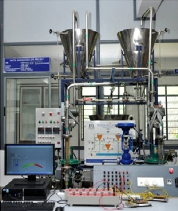
Fig. 15 shows the real time experimental setup of a conical tank process. The level process station was used to conduct the experiments and collect the data. The computer acts as a controller. It consists of the software used to control the level process station. The setup consists of a process tank, reservoir tank, control valve, I to P converter, level sensor and pneumatic signals from the compressor. When the set up is switched on, level sensor senses the actual level values initially then signal is converted to current signal in the range 4-20 mA. This signal is then given to computer through data acquisition cord. Based on the values entered in the controller settings and the set point the computer will take control action and the signal sent by the computer is taken to the station again through the cord. This signal is then converted to pressure signal using I to P converter. Then the pressure signal acts on a control value which controls the flow of water into the tank there by controlling the level.
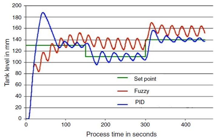
The servo response obtained from the real time conical tank Ta experimental setup is shown in Fig. 16. The results show the comparison of servo response by the FLC and PID controller with setpoint. From the response, it is apparent that the fuzzy controller provides better results when compared to the conventional PID controller.
9. Conclusions
Unlike some fuzzy controllers with hundreds or even thousands of rules running on dedicated computer systems a unique FLC using a small number of rules and straightforward implementation is proposed to solve a class of level control problems with unknown dynamics or variable time delays commonly found in industry. Additionally the FLC can be easily programmed into many currently available industrial process controllers. The FLC simulated on a level control problem with promising results can be applied to an entirely different industrial level controlling apparatus. The result shows significant improvement in maintaining performance over the widely used PID design method in terms of oscillations produced and over-shoot. As seen from the graph the rise time in case of PID controller is less, but oscillations produced and overshoot and settling time is more. But in case of fuzzy logic controller, oscillations and overshoot and settling time are low, so FLC can be applied where oscillations cannot be tolerated in the process. The FLC also exhibits robust performance for plants with significant variation in dynamics. Here FLC and PID both are applied to the same exacting modeled level control system and simulation results are obtained. PID would not have taken care of the unknown dynamics or variable time delays in the system, if the techniques been applied to a system whose exact system dynamics were not known, Fuzzy logic provide a completely different, unconventional way to approach a control problem. This method focuses on what the system should do rather than trying to understand how it works. One can concentrate on solving the problem rather trying to model the system mathematically, if that is even possible. This almost invariably leads to quicker, cheaper solutions. And also using Kalman filter provides more precise results so that controller with Kalman algorithm can be used in noisy environments. This research work can be extended by using the robust extended Kalman filter to effectively use the controller in noisy environments.

