


 text new page (beta)
 English (pdf)
 Article in xml format
 Article references
 Send this article by e-mail
 Cited by SciELO
  Similars in
SciELO
Similars in
SciELO 
 Permalink
1. Introduction
WSNs consist of sensor nodes that are placed in close proximity to, or within the phenomena they observe, according to specific measurement requirements, whilst communicating with other nodes or network access points (Hou & Bergmann, 2010). A true-to-type WSN sensor node consists of a suitable sensor or transducer, a microprocessor to execute trivial logic operations or complex programmes, an RF transceiver to access the network and a suitable power supply (Gungor & Hancke, 2009).
WSNs have been successfully applied in environmental and temperature monitoring (Carullo, Corbellini, Parvis, & Vallan, 2009), machine monitoring (Flammini, Marioli, Sisinni, & Taroni, 2009), energy monitoring (Lu & Gungor, 2009), and increasingly in the fields of optical character recognition OCR (Korber, Wattar, & Scholl, 2007) and thermography (Fluke, 2007).
Thermography measures the temperature of the entire picture that the charged-coupled device (CCD) has captured. For example the Ti-300 infrared thermography imager manufactured by Fluke can be applied in a typical industrial solution to monitor and inspect furnaces and boilers wirelessly using its proprietary ‘SD-wireless’, on-board 802.11 g/n interface (Fluke, 2008). The imager provides a real-time video image and thermographic analysis of the temperature distribution inside the combustion chamber or boiler to Android/Linux nodes. This information is crucial for process control and preventative maintenance procedures, but it requires broadband capability for networked transmission.
ISM band, OFDM WLANs are the proposed solution for WSNs that require broadband operation with committed information rate and predetermined class of service. Two industry measurement standards for data throughput, RFC2544 (Giguère, 2008) and ITU-T Y.1564 (ITU, 2016), are applicable. The terms committed information rate (CIR), excess information rate (EIR) and class of service (CoS) are defined by the Metro Ethernet Forum (MEF, 2006) and by the ITU-T in Y.1564.
CIR and EIR are specifically defined by Y.1564, in terms of measurement philosophy and methodologies, as the acceptable parameters in the method to determine service performance levels that conform to modern industrial and commercial service level agreements. It therefore appears logical that modern IEEE 802.11a/g/n systems that transport TCP/IP Ethernet services for industrial solutions should be evaluated according to the same ITU-T Y.1564 standards. It should be noted here that 802.11b is not an OFDM-based system, but that 802.11a/g/n OFDM systems are backward compatible with 802.11b (Paulraj, Nabar, & Gore, 2003).
Multiple-input multiple-output orthogonal frequencydivision multiplexing (MIMO-OFDM) wireless technology appears to fulfil the requirements of industrial WLANs (Giguère, 2008). MIMO-OFDM is considered a most interesting development in the field of broadband wireless technology because it is extremely tolerant to multi-path propagation and frequency selective fading. A major advantage of an OFDM-based 802.11a/g/n gateway router, for WSN use, is its 3G/LTE Internet connection capability that facilitates a global communication connection (Liu & Li, 2005), seamlessly connection dissimilar operating systems across dissimilar networks. A far-reaching application in mind is that Android/Linux-based IWSNs can be deployed, operated and controlled from anywhere on the globe.
Performance gains may be made in OFDM systems by the application of more than one antenna at either or both connecting points of the wireless link (Bolcskei, 2006). Multiple antennas can be used to effect interference cancellation and may also be used in coherent combining techniques to obtain diversity and array gain. An additional fundamental channel gain is realized by the use of multiple antennas in a MIMO configuration at either/both sides of the link that improves spectral efficiency.
Performance gains may also be made in OFDM systems by the application of a higher gain antenna at either or both connecting points of the wireless link (Ide, Kingsley, O’Keefe, & Saario, 2005). Higher gain antennas like log periodic types are usually highly directional with a beam width of 15◦-20◦ in sector specific direction (azimuth). Attention is drawn to vertically polarized omnidirectional antennas with higher gain, such as the multiple-element collinear array, (Karlsen, 2009) which will only operate satisfactorily in the horizontal plane.
Exceptional performance gains may be made by selecting the appropriate technology that is available to the industry (National Instruments, 2016). For example, a trend observed in both the automotive and military industries is to make use of commercial off-the-shelf (COTS) technology, repackaged to IP65 standards, as opposed to development of turnkey systems from the ground up.
This approach holds many advantages for industrial electronics and informatics practitioners because of time and cost savings related to the measurement platform. For the same reasons, the application of Android/Linux-based platforms has become prolific (National Instruments, 2016). These devices incorporate mostly 802.11a/g/n compatible WLAN capabilities, as well as multiple connectivity options. Their capabilities to connect dissimilar operating systems across dissimilar networks place them functionally on par with OSI model, level 7 gateways.
The latest commercial gateway/routers operate in both ISM frequency bands of 2.4 GHz and 5.8 GHz in the WLAN, so providing frequency diversity. Each frequency band is utilized by two omnidirectional transceivers, hence providing a degree of space diversity, as well as noise cancellation. The gateway employs a so-called ‘hotstick’ USB modem to connect the WLAN to the Internet service provider, typically in a licenced frequency band such as 3.8 GHz.
However, a related problem is to define the degree to which the network can be improved in terms of its service level as a result of performance optimization attempted by the user (Akerberg, Gidlund, & Bjorkman, 2011; Bello, Mirabella, & Raucea, 2007; Sun, Akyildiz, & Hancke, 2011). Advantages for industrial electronics and informatics practitioners from this approach are time and cost savings related to the set-up and operation of the measurement platform.
1.1. Research problem, objective and contributions
The results of bit-rate testing by pattern transmission may be misleading if one considers a phenomenon we shall refer to as the ‘service level differential zone’ (SLDZ) of an OFDM WLAN. The SLDZ of an OFDM WLAN was observed in an industrial environment during preliminary transmission tests that were conducted by the authors in 2007, in preparation of an engine test bench for the purpose of (destructive) diesel engine testing. This form of engine testing requires remote temperature monitoring of the engine components because of the mechanical risks of engine failure which include flying shrapnel and hot oil ejection.
It was observed that the OFDM network will maintain broadbandwidth transmission (video and audio soundtrack) with a node, up to a certain distance away from the access point (AP), as the separating range (r) is increased.
At a range r ne (never exceeded) from the AP, the signal is suddenly compromised with little or no warning by video transmission quality. The node now has to move back a certain distance towards the AP to r max in order to regain transmission. This distance moving back was observed to be a considerable percentage of the total apparent transmission range r ne. It is this considerable range between r max and r ne that we shall refer to as the SLDZ.
The quality of service (QoS) level of a network cannot be accurately determined when nodes are deployed within (or outside) the SLDZ of the network. The SLDZ appears to conform to the magnetic hysteresis phenomenon and underlying physical laws that describe it, for example the Jiles and Atherton (JA) model of hysteresis (Carpenter, 1991).
This paper formulates the hypothesis that connected bandwidth (BW) in Mbps is directly proportional to the power density in W/m2 of the radio frequency (RF) wave, or conversely to the electric field strength (E) of the RF wave in V/m, at the receiving node. Connected bandwidth refers to digital bandwidth, as opposed to analogue bandwidth, which is the frequency range between the half power points of an electromagnetic energy wave. This implies that the connected BW will decrease at the same rate as the power density or the electric field strength of the RF wave, until the decline in signal-to-noise ratio (SNR) results in the termination of streaming wireless communication.
Testing the above-mentioned hypothesis positively is a research goal that motivates the application of the well-known inverse-square law of radiated power, in conjunction with effects of the phenomenon termed here as the service level differential zone. The consideration of the service level differential zone is a novel approach that provides the methods and mathematical building blocks, which are required to solve range, and capacity-related issues of wireless systems (Girs, Uhlemann, & Björkman, 2012).
This paper proposes a method to determine the excess information rate (EIR) and the committed information rate (CIR) by detection, using the SLDZ dynamic hysteresis phenomenon. This technique is combined with scaled video streaming to represent the user defined throughput bandwidth. Previous methods used the file transfer protocol (ftp) method which was not accurate because not all the key performance indicators (KPIs) are considered namely latency and jitter. The d-CIR (detected CIR) provides a quality of service reference, which conforms mostly to the ITU.Y-1564 test philosophy.
This paper contributes the scientific equations and methods that are required to estimate wireless network capabilities, variations and performance during industrial deployment or field tests. With these it becomes possible to qualify OFDM WLANs in terms of their service performance according to acceptable standards such as Y.1564, which is a key requirement for industrial applications.
An extended research goal of this study is to devise a method to compare different OFDM WLAN data links in terms of their performance. An acceptable range performance parameter is required when considering improvement to the link quality, because it will determine the maximum extent to which the link budget can be increased.
The study proposes the typical radio range parameters namely sensitivity and SINAD (signal to noise and distortion ratio) to express OFDM WLAN dynamic range performance. These are mostly used in the specialized field of radio communications. These parameters can be derived from the d-CIR and d-EIR using the SLDZ detection method previously described in this paper.
A method is exploited to determine the excess information rate (EIR) and the committed information rate (CIR) according to the (ITU) and (MEF) by detection, using the SLDZ dynamic hysteresis phenomenon, and to equate these to the radio range characteristics of the physical layers under test. This technique is combined with scaled video streaming to represent the user defined throughput bandwidth. The d-CIR (detected CIR) provides a quality of service reference, which conforms mostly to the ITU.Y-1564 test philosophy.
1.2. Analytical approach: the free space radiation model
In order to determine the characteristic transmission curve of the wireless link under test, samples of connected bandwidth BW are drawn at diminishing range intervals. These samples are then processed with MS Excel to produce a logarithmic trend line, depicting connected BW as a function of range in metres.
The stepped curve response of the transmission characteristics makes more accurate reading intervals difficult and pointless. The connected bandwidth level at each respective range section is maintained until the firmware switches over to the next lower (or higher) BW setting. The BW switching criteria are not published by the manufacturer so that the effects can only be observed, but not clearly explained.
A simple solution is a method to smooth the stepped curves by using logarithmic trend modelling such as Excel or MatLab functions. More meaningful readings can then be made graphically, and the resulting graph function may be used to calculate range-corresponding BW variations.
The point source radiator or isotropic antenna has to be considered in the study of the radiated field from any antenna, when line-of-sight transmission is considered. Practical antennas and their performance are often referenced in terms of this basic radiator.
1.3. Derivation of the range equations
Energy radiates equally in all directions from the isotropic antenna; therefore, the spherical radiation pattern in any plane is circular, for example in the ground plane. The typical isotropic radiator is supplied with a power of P watts at the origin O. The power flows outward from this point and through the spherical surface S, which has a radius r. The intensity of radiation, i.e., the power density P D at point I can be defined as:
This equation illustrates the effects of the inverse square law of irradiance: at twice the range (2 × r), with P at a constant, the power density P Di decreases by a factor of four or by −6 dB. Also, to obtain the same P Di at double the range (2 × r), the power P would have to increase fourfold or by +6 dB, irrespective of the number of antennas used (Wolnicki, 2005), as confirmed by Wavion’s MIMO enterprise AP equipped with six +6 dBi antennas.
Maxwell’s theories define the relationship between the power density P Di and the E-field and H-field vectors as follows (Maxwell, 2011):
The absolute magnitude of the power density or intensity of irradiation is thus:
(where Ei is the electric field strength of irradiance and the impedance of free space is 120 ohm, which is approximately 377Ω.
According to the inverse square law, the ratio of two power densities at their respected ranges from the source of radiation can be expressed as the link budget variation, in dB:
Manipulation yields:
Since P Di =Ei 2/120π (Maxwell, 2011):
But according to the hypothesis, the electric field strength Ei is directly proportional to the connected bandwidth BW:
When the bandwidth remains a constant (BW 1 = BW 2), then the ratio of the two respective ranges may be expressed as:
(This is the equation proposed for the analytical processing of data samples)
Also, when the range remains a constant (r 1 = r 2), then the ratio of two bandwidths may be expressed as:
With Eqs. (3) and (4) it becomes possible to predict throughput variations in terms of relative RF link budget (in dB), and to qualify OFDM WLANs in terms of their service performance according to acceptable standards such as Y.1564, which is a key requirement for industrial applications.
1.4. Research objective
The main research objective of this study was to devise a simple method to analyze and estimate the performance of an ISM-band, OFDM-based, WSN data link. We compare the transmission characteristics before and after signal intensification or attenuation is configured, and relate the differences in terms of the RF link budget (in dB), by the application of Eq. (3). Results are then presented for discussion.
2. Methods and test environment
This section describes the experimental methods and the conditions under which the test results were obtained so that the experiments may be easily replicated for continuous review and investigation. Then, the analytical approaches are briefly reviewed before the data analysis method is described.
Testing is in accordance with the neural black-box method combined with the mathematical approach of functional approximation. The digital inputs to the entire system are compared with the analogue video and audio output obtained in terms of observed quality. The inner hardware of the node or the physical layer cannot be manipulated by the user, therefore it remains irrelevant to this study. However, different physical layers can now be compared with one another in terms of functional performance.
The test topology is shown in Figure 1.1(a)-(c). The test range is shown in Figure 1.2. The typical OFDM test network consists of two mobile computers and an ISM 802.11.g access point (AP) router. The 802.11g system was used as an example because this system version (g) was already well developed in terms of industrial packaging and antennas/accessories available. We also used 802.11g as an example because of interest in the results obtained from single transceiver systems, as opposed to multiple transceivers as in MIMO operation. The fact of the matter is that the similar results will (predictably) be obtained when repeating these tests with any of the IEEE ratified systems 802.11a/g/n.


Figure 1.1 depicts the network options for testing. The server node used option (a) for Experiment 1, option (b) for Experiment 2 and option (c) for Experiment 3. Typical ISM band OFDM network variations were deployed for streaming video transmission. Performance results were measured and are presented here as connected bandwidth (BW) in Mbps, as a function of transmission range (r) in metres. The server node is directly connected to the AP via Cat 5 cable, and also controls the AP adapter settings with a browser-based guided user interface (GUI). For the mobile node’s adapter, Intel PROSet Wireless adapter software is used with the mobile node because it is freely available and easy to use. The installation of this additional software enhances the functionality and user perception of the measurement experience.
Radiation measurements normally have to be conducted in an anechoic chamber or open-space antenna measurement range. Results otherwise obtained will be regarded as conduction measurements rather than radiation measurements, and are therefore not considered here.
Since the method described here is intended for actual field use and refers to the SINAD parameter (ratio of signal to noise and distortion), the results were required to include the effects introduced by external noise and distortion. The transmission tests were therefore conducted on an old cricket pitch, as shown in Figure 1.2, providing a relatively large open space with an evenly flat ground plane.
Figure 1.2 shows the plan area of the transmission test range. The approximate latitude and longitude of the test station is indicated, as well as the imaginary range line and markers. The d-CIR and d-EIR ranges for the three transmission series in Figure 3 are also indicated.
Video transmission commences when the mobile node runs the file in the server node’s share folder with Windows’ media player. The use of a predetermined video bit-stream is applied in a test detection technique: If the video stream at a specific prescaled rate has no perceptual impairment in terms of sound or picture, it conforms completely to the agreed CIR. If any noise or video distortion is perceived, it means the key performance indicators (KPIs) are compromised and the video stream does not conform to the agreed CIR.
The video bit-stream rate was predetermined to represent the committed information rate (CIR) or agreed QoS throughput, set at nominally 600 kbps maximum for the experimental requirement. This was achieved by selecting a suitable length video clip and scaling the frame rate down in H.264 with Apple’s video editing software until the desired bitrate was obtained. The resulting audio/video interleaved (AVI) file was then saved on the server node in a shared folder.
2.1. Experimental methods
The first set of experiments focused on passive testing. This means the determination of the transmission characteristics for a throughput of 600 kbps with any variations imposed in a passive (i.e., inactive) manner, as compared with the standard lowcomplexity (+1 dBi) antenna characteristics as in Experiment 1.
These characteristics are compared to transmission characteristics when using an antenna with a higher gain characteristic (Willig, 2008), for example a vertical (+6 dBi) collinear design for 2.4 GHz in Experiment 2. The test was repeated using two inline resistive attenuators of 6 dB each in conjunction with the +1 dBi antennas in Experiment 3.
The second set of experiments focused on active testing. This means that the transmission characteristics for a throughput of 600 kbps were determined for different settings of transmitted power levels, which were electronically controlled by Intel’s PROSet Wireless software. The transmission characteristics of a typical 802.11 g single transceiver network operating at 20% of maximum power were determined in Experiment 4. The test was repeated for a power setting of 80% of maximum power in Experiment 5.
2.1.1. Experiment 1: Test network service reference
Experiment 1 determined the service reference for the electronics that was utilized. The electronics used for this test employed OFDM MIMO technology, manufactured by Belkin, AP model 802.11g+ MIMO with fixed transmit power at +17 dBm. With the mobile node equipped with the matching Belkin USB g+ MIMO modem, the two transceiver system enabled a near range data connection rate of 108 Mbps.
The set-up for Experiment 1 is shown in Figure 1 (a). After starting the video transmission, the BW was recorded at suitable distance intervals whilst increasing the transmission range to the point of total signal deterioration, as shown in Figure 2. This point is marked as the detected excess information rate (dEIR) range. The transmission range was then reduced until video transmission restarted. This point was marked as the detected committed information rate (d-CIR) range. The SLDZ is the range between d-CIR and d-EIR.

Figure 2 contains the data collected during Experiment 1, in a graph generated with the aid of Excel. The indicated d-CIR and d-EIR are for a test bit-rate of 600 kbps that is continuously monitored in terms of four key performance indicators namely bandwidth, latency, jitter and errors. Note the range at which transmission fails (72 m) corresponds to approximately 6 Mbps.
When reducing the transmission range, the transmission restarts at 55 m at approximately 18 Mbps. Our method to use a trend-line is applied so that more accurate information may be extracted from the stepped transmission curves, or by using the equation y = −26 ln(x) + 125.6 also generated with the use of Excel. These stepped curves are due to the manufacturer’s (Intel) internal algorithms that are contained in the firmware of the OFDM WLAN physical layers, which can be smoothed with the use of external software packages like Excel.
The SLDZ manifests itself in the same manner as a typical hysteresis curve (Carpenter, 1991); transmission failing suddenly at d-EIR and restarting back at d-CIR. This pattern will repeat as the mobile node approaches or recedes from the access point AP across the SLDZ.
2.1.2. Experiment 2: Test network with improved service reference
Experiment 2 determined the improvement in the service reference for the electronics that was utilized. However, instead of the standard +1 dBi antennas, the AP was equipped with two +6 dBi antennas as shown in Figure 1 (b). The mobile node was equipped with the matching Belkin USB g+ MIMO modem. The data collected during Experiment 2 is depicted in Figure 3 as (b) Transmission +6 dBi.

Fig. 3 Transmission characteristics for MIMO test network with (a) +1 dBi antennas, (b) +6 dBi antennas and (c) 6 dB attenuators in-line with +1 dBi antennas.
Figure 3(b) indicates the test results obtained with +6 dBi antennas instead of +1 dBi, which means the link budget was improved by 5 dB.
2.1.3. Experiment 3: Test network with reduced service reference
Experiment 3 indicates the reduction in the service reference for the electronics that was utilized, as a control procedure. However, instead of the standard +1 dBi antennas, the AP was also equipped with two 6 dB attenuators fitted in-line with each antenna as shown in Figure 1.1(c). This means the link budget was reduced by 6 dB.
The set-up for Experiment 3 is shown in Figure 1.1(c) and the data collected during the experiment is depicted in Figure 3 as (c) Transmission −5 dBi.
2.1.4. Experiment 4: Test network with node RF power at +11 dBm
Experiment 4 determined the service reference for the electronics that was utilized when operating a node at 20% of maximum power. The electronics used for this test was an 802.11g AP router with single transceiver manufactured by DLink operating at +18 dBm.
The wireless adapter control software on the mobile node made it possible to set RF power in 20% decrements from maximum (+18 dBm/63 mW) to zero. For this test the mobile node RF power was set to 12.6 mW or +11 dBm. The single transceiver system enabled a near range data connection rate of 54 Mbps.
2.1.5. Experiment 5: Test network with node RF power at +17 dBm
Experiment 5 determined the service reference for the electronics that was utilized when operating a node at 80% of maximum power. For this test the mobile node RF power was set to 50 mW or +17 dBm. The single transceiver system enabled a near range data connection rate of 54 Mbps.
The set-up for Experiment 4 and Experiment 5 is essentially indicated in Figure 1.1(a) but with a single antenna on the AP and using the internal RF modem situated on-board the mobile node. The results of the active tests are indicated Figure 4.
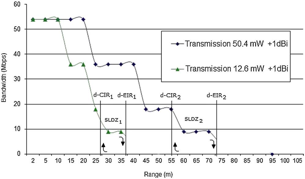
Fig. 4 Single transceiver transmission characteristics with actively controlled transmit power, indicating typical stepped curves for two series.
In Figure 4, the first series presents the transmission results with RF power set to +11 dBm (12.6 mW), and the second series of results are for RF power set to +17 dBm (50.4 mW). Figure 4 thus indicates the transmission range variation when the RF output power setting is adjusted by +6 dB, which is four times original setting.
2.2. Comparative testing
This section briefly reviews the methods and conditions under which the comparative test results were obtained, so that the experiments may easily be replicated for continuous review and investigation.
The test topology is shown in Figure 5 (a) and (b). The typical OFDM test network consists of two mobile computers and an ISM 802.11.g access point (AP) router.

The server node used option (a) for Experiment 6 and for Experiment 7. The mobile node in Experiment 6 used an external USB modem. Nevertheless, a different manufacturer’s mobile node was used for Experiment 7, equipped with an internal 802.11a/g/n physical layer, as in Figure 5 (b).
Experiment 6 focused on the determination of the transmission characteristics for a throughput of 600 kbps with two standard low-complexity (+1 dBi) antennas in a MIMO configuration as depicted in Figure 5 (a). These characteristics are compared to the transmission characteristics obtained during Experiment 7, when using a single transceiver (Txcvr) AP as indicated in Figure 5 (b). Note that, the RF power level for both tests, were set to equal levels at +17 dBm each.
2.2.1. Experiment 6: MIMO test network service reference
Experiment 6 determined the service reference for the electronics that was utilized. The electronics used for this test employed OFDM MIMO technology, manufactured by Belkin, AP model 802.11g+ MIMO with fixed transmit power at +17 dBm. With the mobile node equipped with the matching Belkin USB g+ MIMO modem, the two transceiver system enabled a near range data connection rate of 108 Mbps. The set-up for Experiment 6 is shown in Figure 5(a).
Figure 6 contains the data collected during Experiment 6, in a graph generated with the aid of Excel. The indicated d-CIR and d-EIR are for a test bitrate of 600 kbps that is continuously monitored at the receiver node in terms of four key performance indicators namely bandwidth, latency, jitter and errors. Note the range at which transmission fails (72 m) corresponds to approximately 6 Mbps. When reducing the transmission range, the transmission restarts at 55 m at approximately 18 Mbps. A method to use a trend-line is applied so that more accurate information may be extracted from the stepped transmission curves.

2.2.2. Experiment 7: Single transceiver test network service reference
Experiment 7 determined the service reference for the electronics that was utilized when operating a link with a singletransceiver node. The electronics used for this test employed OFDM MIMO technology, manufactured by Belkin, AP model 802.11 g+ MIMO with fixed transmit power at +17 dBm.
Nonetheless, the mobile node for this test was equipped with a single-transceiver system that enabled a near range data connection rate of 54 Mbps. The transmission results for Experiment 7 are shown in Figure 7.

2.3. Analytical approach and methodology to comparative testing
The analytical approach is mathematically simplified, in order to accommodate a much wider spectrum of industrial and scientific users who may not all be expert mathematicians. All data was first captured into MS Excel, and then processed to produce logarithmic trend-line equivalent curves with corresponding mathematical expressions. The resulting trend-line’s y-intersect was then adjusted until the curve intersected with the last minimum recorded (70 m) at the distance boundary, as shown in Figure 6 for the MIMO test network and Figure 7 for the single transceiver.
With the aid of the logarithmic trend graph indicated in Figures 6 and 7, the BW values corresponding to the d-CIR and d-EIR can be more accurately extracted from the data collected. As indicated, the transmission characteristics were measured in decreasing steps as determined by the wireless adapter’s onboard firmware and algorithms. The result is a rather erratic stepped curve with more than one range value for each BW value below 54 Mbps.
According to the trend graph in Figure 6 (which can also be described by y = −26.6ln(x) + 125.6 for the section of interest), the BW value at a range of 55 m (d-CIR) is 19 Mbps. The trend graph extends in range up to the last measured BW value before transmission terminated.
For the section of graph beyond 70 m, the interpolation method used here to estimate the BW at 72 m (d-EIR) is by assuming a straight line graph section between 70 m (9 Mbps) and 75 m (0 Mbps). If 72.5 m corresponds to 4.5 Mbps, then the interpolated bandwidth at 72 m is approximately 5 Mbps.
Considering the single transceiver’s characteristics and resulting logarithmic trend graph as depicted in Figure 7, y = −14.17ln(x) + 71.356, the d-CIR range corresponds to a connected bandwidth value of 14.5 Mbps and the d-EIR range a value of 2.5 Mbps.
3. Results and data analysis
In the method followed to test the hypothesis, samples were drawn from the data collected during experimentation presented in Section 2. After starting the video transmission, the BW data was recorded at suitable distance intervals whilst increasing the transmission range to the point of total signal deterioration, as shown in Figure 3. These data samples were then processed with an Eq. (3) derived in the previous Section 1.3, which is based on the inverse square law of radiated power.
The equation reveals the relationship between range variation (r 1/r 2) and signal strength (dB) when the bandwidth (BW) is constant (at 600 kbps). Each of the processed results is then compared with the expected value.
3.1. Passive test data analysis
Considering Figures 2 and 3, Table 1 compares the results obtained with the standard +1 dBi antennas to the results obtained with the +6 dBi antennas, thus a total link budget variation of +5 dB.
Table 1 Transmission results +1 dBi antenna vs. +6 dBi antenna.
| Measured result | Calculated result dB=(20Logr2/r1) | Expected result dB=(+6 - 1 dB) | ||
|---|---|---|---|---|
| Data rate | r 1 | r 2 | ||
| 36 | 25 | 45 | 5.11 | 5 |
| 36 | 32 | 57 | 5.01 | 5 |
| 36 | 40 | 70 | 4.86 | 5 |
| 18 | 45 | 75 | 4.43 | 5 |
| 18 | 50 | 90 | 4.81 | 5 |
| 18 | 55 | 100 | 5.19 | 5 |
| CIR | 57 | 102 | 5.05 | 5 |
| 9 | 65 | 115 | 4.95 | 5 |
| 9 | 70 | 125 | 5.03 | 5 |
| EIR | 72 | 127 | 4.93 | 5 |
| Standard deviation | 13% | - | ||
Considering Figures 2 and 4, Table 2 compares the results obtained with the standard +1 dBi antennas to the results obtained with 6 dB attenuators set fitted in-line, thus a total link budget variation of −6 dB.
3.2. Active test data analysis
Considering Figure 5, Table 3 compares the results obtained with the RF transmit power set to 50.4 mW (+17 dBm); to the results obtained with the RF transmit power set to 12.6 mW (+11 dBm). This represents a 6 dB difference in power level, or a 1-4 power ratio.
3.3. Standard deviation
The standard deviation for each of these three series in Tables 1-3, are respectively estimated at 13%, 4.2% and 16.6%. This is regarded as excessive in the first and last cases and can be attributed to the stepped transmission curves.
3.4. Processing data to improve standard deviation
In a second method of data analysis, collected data samples are processed to produce a logarithmic trend-line, in order to reduce the standard deviation i.e. accuracy of the measurements. The following Figure 8 indicates a logarithmic trend-line for the series +6 dBi shown in Figure 3(b).

Using the logarithmic trend-line, specific values can be extracted for the respective data rates 36 Mbps, 18 Mbps, 9 Mbps, d-CIR and d-EIR. Similarly, specific values were extracted from the series in Figure 2, and the two sets of processed values can again be compared in terms of the expected results, as shown in Table 4 below.
4. Discussion
4.1. The hypothesis
The hypothesis suggests that connected bandwidth (BW) in Mbps is directly proportional to the electric field strength (E) in V/m, or to the power density (PD) in W/m2, of the RF wave at the receiving node.
To test the hypothesis, several experiments were conducted. The hypothesis was confirmed by the experimental results obtained and presented in this study, since they correlate with expected values. The positive testing of the hypothesis suggests that connected bandwidth BW in Mbps is directly proportional to the relative signal strength in dBm, which is the preferred expression of signal power level.
Positive testing of the hypothesis motivates the application of the inverse squared law of radiated power (or irradiation) as a mathematical tool to estimate information rate variations in ISM band OFDM wireless Ethernet networks, as applied in industrial wireless sensor networks.
By using a video bit stream of a pre-determined rate to specify the required committed throughput, the service level differential zone SLDZ can easily be measured and the CIR and EIR for each network option can be detected. Once the d-CIR and dEIR transmission ranges for the network options are known, these values can be used in conjunction with a simple set of Eqs. (3) and (4) to estimate range or bandwidth variations in network performance, in terms of relative link budget in dB.
The observation of a video stream in order to evaluate network key performance indicators (KPIs), namely bandwidth, latency, jitter and errors, provides a fast, intuitive and easily interpreted method to confirm the CIR under actual operational conditions. It appears easier to use BW to express relative variations in signal strength in dB, because the measurement of RSS in dBm requires special test equipment and an in-depth knowledge of test and measurement w.r.t. resolution bandwidth measurements. BW readings may be obtained from on-board instrumentation such as Window Task Manager (Networking pane) or PROSet Wireless freeware from Intel.
4.2. The digital SINAD ratio
An interesting phenomenon initially observed is that the CIR (in the example’s case 600 kbps max) requires a minimum of approximately ten times the connected bandwidth, to a maximum of approximately thirty times the connected bandwidth, to reconnect or reset. These limits are determined by the manufacturer’s firmware, situated on the radio chipset. This means the 600 kbps CIR fails at a connected bandwidth value below 6 Mbps, and reconnects or recovers from reset at approximately 18 Mbps connected bandwidth.
With specific reference drawn to the observation above, the signal-to-noise-and-distortion ratio (SINAD) is considered because it is an indicator of the quality of the signal that is transmitted from a communications device, and is often defined as:
By functional comparison, the d-EIR is the transmission range at which the signal level of the CIR has deteriorated to the point that it is overcome by the noise and distortion level. Conversely, the d-CIR is the transmission range at which the CIR signal level is at a sufficiently higher ratio elevated above the noise and distortion level for acceptable video transmission. This situation relatively represents the digital SINAD ratio which can be calculated from the proposed equation:
With reference to the results of the passive tests in Figures 2-4, the SINAD for each characteristic was calculated with values obtained from the Excel trend-line method as in Figure 2. For example, for the curve Tx +1 dBi:
For the curve Tx +6 dBi, using the same method, the SINAD is calculated at 13.18 dB, and for the curve Tx −5 dBi the SINAD is 15.44 dB. Acceptable results were noted for Tx +1 dBi and Tx +6 dBi, since the SINAD required for microwave frequency is expected to be slightly higher than the 12 dB recommended for VHF.
A higher than expected SINAD of 15.44 dB was noted for the Tx −5 dBi curve to produce acceptable results. The additional signal level that is required to produce acceptable results is probably to overcome additional return loss because of mismatch. The mismatch probably occurs as a result of the additional connectors introduced to the system by the attenuator pads.
4.3. Comparative test results
The sensitivity specification of the first mobile node in Figure 5(a) as a radio receiver, for the transmission characteristics shown in Figure 6, can also now be estimated as 19 Mbps for a 13.35 dB SINAD at throughput CIR of 600 kbps. (18 Mbps may be used being the closest standard BW value that the network can connect, for an approximated value of 13 dB SINAD).
For the second example, the SINAD can be calculated for the curve depicted in Figure 7 by the same method:
Again, the sensitivity specification of the second mobile node in Figure 5(b) as a radio receiver can now be estimated as 14.5 Mbps for a 13 dB SINAD at a throughput CIR of 600 kbps.
The results obtained by the study, for two dissimilar physical layers transporting the same CoS traffic, can now be tabulated for brief discussion (Table 5):
Table 5 Comparison of experiment 6 - mimo dual transceiver and Experiment 7 - single transceiver.
| MIMO Experiment 6 | Single transceiver Experiment 7 | |
|---|---|---|
| SINAD | 13.35 dB | 13.01 dB |
| Sensitivity | 19 Mbps for approx. 13 dB SINAD at CIR = 600 kbps | 14.5 Mbps for approx. 13 dB SINAD at CIR = 600 kbps |
It is noted with interest that the single transceiver has a much improved sensitivity rating. This was not clear from initial measurements, because the same d-CIR range was measured. However, with the use of the logarithmic trend graph it became possible to estimate the corresponding data rate with closer accuracy and clearly reveal the difference in physical layer characteristic features.
5. Conclusion
The study introduces WSNs to ISM-band OFDM WLANs, with specific reference to thermography and Android-based computer technology.
A novel method to estimate a specified committed information rate in terms of range and link budget is positively tested against expected values. These capabilities render OFDM WLANs operating within ISM bands an extremely useful communications transport medium for industrial wireless sensor networks, and specifically for cutting edge Android nodes with Linux-based operating systems.
A hypothesis is proposed that connected bandwidth in OFDM WLANs is directly proportional to the relative RF signal strength. The concept is mathematically proved by a heuristic statistical analysis approach, whereby data collected from transmission characteristics are compared with expected results, when the signals are intensified or attenuated to specifically known values. A method is revealed whereby collected data are processed in order to substantially improve the accuracy of the measurements.
Comparative studies by physical experimentation revealed that mobile nodes can be individually tested in terms of their respective SINAD parameters, as well as their sensitivity parameters, without connecting external test equipment. With these parameters available, mobile Android/Linux computer nodes can in future be qualified for industrial use in terms of their throughput performance, which is a key requirement for service level agreements (SLAs) which incorporate the ITU-T Y.1564 and EtherSAM test methodologies.

