


 nueva página del texto (beta)
 Inglés (pdf)
 Artículo en XML
 Referencias del artículo
 Enviar artículo por email
 Citado por SciELO
  Similares en
SciELO
Similares en
SciELO 
 Permalink
1 Introduction
Measurement of sound absorption coefficient is considered to be important in determining the acoustic properties of materials considered for use in noise control. Sound absorption coefficient is a quantity that represents the percentage of sound absorbed by a material. This is measured using the phenomenon of reflection of sound waves. Sound waves are generated within a medium and transmitted towards the test sample. By measuring the incident and reflected waves, reflection coefficient and hence the acoustic impedance can be calculated. The two standard methods for determining the absorption coefficient are Standing Wave Ratio (SWR) (Iso, 1996) method and transfer function method (International Organization for Standardization, 2001). The standing wave pattern and its pressure measurement are used in the former, whereas in the latter, transfer function is used. A method to measure sound absorption coefficient of acoustical materials used as wall or ceiling treatments is proposed in (Iso, 2003), providing results at random incidence. An optimization method based on flow resistivity to improve reproducibility is proposed in (Jeong & Chang, 2015). A new technique to measure sound absorption coefficient using sound intensity probes is discussed in (Bonfiglio, Prodi, Pompoli, & Farina, 2006). Another method that uses echo impulse technique to measure acoustic impedance is elaborated in (Garai & Pompoli, 2001), which requires further post processing of results to obtain accurate measurements. The acoustic impedance is generally calculated over a wide range of frequencies and these standard methods introduce errors in the measurement setup. Various procedures to mitigate these errors have been dealt in the literature.
Bias and random errors occur while finding the transfer function between the microphone positions. In (Pilon, Panneton, & Sgard, 2004), the effect of air gap in standing wave tube was discussed with experimental results. The impact of barometric pressure, sample mounting and error in apparatus was studied and an analysis was presented in (Tinianov & Babineau, 2006). The measurement is also affected by dispersion, which can be studied using reproducibility concept (Horoshenkov et al., 2007). These errors were mitigated in (Åbom, 1988) by decreasing the duct length, having a non-reflective source end and having the microphone as close as possible to the source. Also, they investigated that there should be a minimum spacing between the two microphone locations to reduce large errors due to pressure nodes at the microphone location. In (Katz, 2000), to reduce errors, proper location of microphone was determined. In this paper, an additional microphone is used to estimate the precise distance than using a ruler using ISO-method. A verified systematic framework to estimate frequency dependent uncertainties in the complex reflection and normalized acoustic impedance calculations was proposed in (Schultz, Sheplak, & Cattafesta, 2007).
A two microphone three calibration method was proposed in (Gibiat & Laloe, 1990). In this method, impedance of three known devices is connected subsequently and the impedance of the unknown device is calculated by using the three known impedance and the transfer function obtained from the unknown device.
A multiple microphone method was proposed to measure pressure at more than three positions. The acoustic impedance is calculated from the transfer function of a few combinations of microphones. An improved method was proposed in (Cho & Nelson, 2002) using least square curve fitting and optimizing the response of all microphone positions. Here again, multiple microphones were employed to determine various transfer function values and choosing the best.
All the above methods of error correction involve a constructional change in the impedance tube or at least a calibration mechanism, which is not standardized. To overcome the difficulty, a novel intelligence based error correction mechanism is developed based on soft computing techniques. In this paper, error reduction in impedance tube is considered as an optimization problem. Numerous soft computing techniques such as Firefly Algorithm (Nasiri and Meybodi, 2012), Simulated Annealing (Mantawy, Abdel-Magid, & Selim, 1998), Ant colony optimization (Xiao, Zhou, & Zhang, 2004), Artificial Bee colony (Karaboga & Basturk, 2007), Bat and Artificial immune system (AIS) (Taha, Mustapha, & Chen, 2013), have already been applied to different optimization problem. Neural networks have been used in various application areas for error correction and proved to be efficient. In (Ren, Xu, Sun, & Yue, 2011), thermal error correction is carried out using back propagation neural network and rough sets in CNC machine. Error minimization in radio occultation electron density retrieval (Pham & Juang, 2015), wind speed forecast (Zjavka, 2015), colour correction (Zhuo, Zhang, Dong, Zhao, & Peng, 2014) and coordinate boring machine (Yang et al., 2014) with neural networks have been addressed in the literature. PSO is combined with a time difference of arrival algorithm to reduce error in finding emitter location for various applications (Cakir, Kaya, Yazgan, Cakir, & Tugcu, 2014). Calibration of three axis magnetometer is done using Particle Swarm Optimization (PSO) and its variant (Wu, Wu, Hu, & Wu, 2013) by reducing the sensor errors. Various other applications include tool positioning (Mahapatra & Devi, 2013), prediction of geometric errors in robotics (Alici, Jagielski, Ahmet Şekercioğlu, & Shirinzadeh, 2006). To minimize error in impedance tube, soft computing techniques have not been applied yet in the literature. Neural network has been used to model different materials to estimate the sound absorption coefficient (Gardner, O'Leary, Hansen, & Sun, 2003). PSO (Kennedy & Eberhart, 1995) and ANN (Sarle, 1994) have been chosen in this paper, as these two algorithms have already been used successfully in the literature as discussed earlier. The errors arising in the measurement of acoustic impedance due to various reasons is modelled mathematically from sample data available through experiments. Neural network and PSO are designed to reduce the errors, and their results are compared with the standard tube.
2. Impedance tube
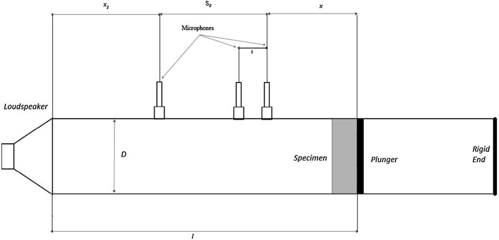
To test the sound absorption coefficient, a transfer function based impedance tube has been developed. One microphone method is employed by using a single microphone at two location successively, thereby avoiding phase mismatch between two different microphones (Allard, 1993). The theory of transfer function method has already been discussed extensively in the literature (Chung & Blaser, 1980a, 1980b). The developed impedance tube along with the entire setup is shown in Figure 1.

2.1. Methodology
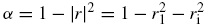
In the proposed methodology, a sinusoidal sound source is used that generates plane waves in the tube. The sound pressure is measured at two locations in close proximity to the sample. The complex acoustic transfer function of the two microphones signal is determined and then used for calculating the normal - incidence complex reflection factor (r ), normal - incidence absorption coefficient (α ) and impedance ratio of the test material. It is found that the frequency range depends on the diameter of the tube and the distance between the microphone positions.
The normal - incidence complex reflection factor can be calculated using the formula
 (1)
(1)
where x 1 , distance between sample and the farther microphone location; Φ r , phase angle of normal incidence reflection factor; H 12 , transfer function from microphone one to two, defined by complex ratio p 2 /p 1 = S 12 /S 21 . H R & H I are the transfer function for the incident wave and transfer function for reflected wave.
The sound absorption coefficient can be calculated as:
 (2)
(2)
2.2. Tube fabrication for transfer - function method
The impedance tube is made from a rigid, smooth, non-porous walls. To avoid vibration resonance in the working frequency range, the walls of the tube are made thick and heavy. The tube is made from brass and the holes for microphones are drilled to the required tolerance of ±0.2 mm. To seal the microphone hermetically, rubber seals are inserted at the holes where microphones are placed. A rigid plunger is fitted at the end of the tube to back the sample material. The rigid plunger is made of mild metal with a thickness of 23.8 mm. A membrane loud speaker is connected at the opposite end of the tube. The surface of the loudspeaker membrane covers two-thirds of the cross-sectional area of the impedance tube. Loudspeaker is contained in an insulating box in order to avoid airborne flanking transmission to the microphones as shown in Figure 2.
2.3. Tube calculation for transfer function method
For sound absorption coefficient measurement, the generated sound signal shall be a plane wave. Therefore, the tube has to be long enough to ensure the development of plane sound waves between sound source and the sample. The standard ISO 10534-2 recommends a tube length of at least thrice the diameter, as non-plane waves will disappear at that distance. A length of at least 10-15 times the diameters is preferred (Seybert, 2010). The upper working frequency is chosen in such a way as to avoid the occurrence of non-plane wave mode propagation and to assure accurate phase detection (RYU, n.d.). The upper limiting frequency f u can be calculated from the following condition.
 (3)
(3)
The inner diameter of tube for this design is d = 104.8 mm which gives the upper liming frequency of f u = 1.8 kHz. The limiting frequency depends on the distance between the microphones, s 0 , as depicted in Figure 2, which should exceed 5% of the wavelength corresponding to the lower frequency interest. Therefore, s 0 determines the lower limiting frequency f l using the following condition.
 (4)
(4)
Additionally, the following condition has to be satisfied.
 (5)
(5)
For the selected distance s 0 = 30 cm, the lower limiting frequency is f l = 58 Hz. A larger spacing between the microphones has been chosen in order to enhance the accuracy of measurement (Suhanek, Jambrosic, & Domitrovic, 2008). The spacing between the sound source and microphone x according to ISO 10534-2 should be
 (6)
(6)
For this study, the spacing between the sound source and microphone is taken as x = 720 mm. The distance x 2 between the test sample and the microphone nearest to it depends on the type of sample. To meet the highly asymmetrical nature of sample, the value is chosen as below.
 (7)
(7)
Finally, the total tube length is given by
 (8)
(8)
3. Systematic and random errors in measurement
Errors in an impedance tube can be classified into intrinsic and extrinsic errors based on the source of the error. Intrinsic errors arise due to the internal parts of the impedance tube including microphone error, specimen mounting error, loudspeaker distortion and duct resonance. Extrinsic errors are due to the instruments used to aid the measurement of acoustic impedance like signal source error, power supply error and errors due to electronic circuitry. The influence of measurement apparatus, related instruments, and the sample material's behaviour causes systematic errors in the readings. Systematic errors include errors intrinsic to impedance tube operation, errors intrinsic to test specimen mounting and errors intrinsic to the measurement instrumentation. It may be due to the attenuation within the tube, probes and structure-borne vibration. Errors in the electronic circuitry also adds to these systematic errors. Random errors are also introduced in the reading due to environmental and operational conditions.
Thermal conduction in the acoustic boundary layer near the tube wall attenuates the wave motion and decreases the standing wave ratio. Backing cavity also plays a role in the measurement of impedance. The impedance measured includes the interaction of test specimen as well as cavity impedance. Systematic errors can be avoided by adjusting the cavity depth for zero reactance. The pressure probe has a finite size and hence introduces a systematic error due to deviation from the Rayleigh end correction value of 0.85 rp. It is thus required to determine the end correction by experimental method before measurement. Mechanical vibrations of the tube also introduce systematic errors, especially at low values of pressure.
4. Error dependencies
The inaccuracies in a tube are due to a number of factors. But some factors may be repetitive. Some of the errors can be corrected using calibration while other errors may vary with the operating conditions of the impedance tube. These errors may require dynamic calibration and can be difficult to correct. IN this paper, in order to improve the accuracy of the results, the dependency of accuracy on measurable parameters is analyzed. It is observed that the quantity of error varies with the frequency of the input signal. The impedance tube produces similar measurements for a material at a given frequency of the input signal. Hence the inaccuracies in the measurements are attributed to the nature of the tube, electronic circuit and other components of the system. The accurate measurement is a function of measured value from the impedance tube and error factor as in Eq. (9).
 (9)
(9)
where α cor is the desired accurate measurement as compared with B&K impedance tube α is the measurement from a standard impedance tube which is accepted to be accurate. Several test materials are collected and their sound absorption coefficients as calculated from standard B&K impedance tube and the developed impedance tube and few samples are shown in Table 1.
Table 1 Sample training dataset.
| F (Hz) | Sound absorption coefficient | ||||||||
|---|---|---|---|---|---|---|---|---|---|
| Glass wool - 1600 g/m2 and 80 mm | Resin felt - 1000 g/m2 and 15 mm | Resin felt - 2000 g/m2 and 30 mm | |||||||
| A | B | Error (%) | A | B | Error (%) | A | B | Error (%) | |
| 80 | 0.050 | 0.065 | 30.0 | 0.020 | 0.022 | 10.0 | 0.035 | 0.038 | 8.57 |
| 100 | 0.066 | 0.071 | 7.21 | 0.018 | 0.019 | 5.56 | 0.031 | 0.032 | 3.23 |
| 125 | 0.086 | 0.099 | 14.4 | 0.021 | 0.022 | 4.76 | 0.040 | 0.043 | 7.50 |
| 160 | 0.115 | 0.121 | 4.95 | 0.031 | 0.031 | 0.00 | 0.057 | 0.060 | 5.26 |
| 200 | 0.117 | 0.151 | 28.5 | 0.038 | 0.036 | 5.26 | 0.075 | 0.077 | 2.67 |
| 250 | 0.136 | 0.145 | 6.40 | 0.049 | 0.048 | 2.04 | 0.097 | 0.103 | 6.19 |
| 315 | 0.336 | 0.341 | 1.46 | 0.06 | 0.068 | 13.3 | 0.127 | 0.128 | 0.79 |
| 400 | 0.540 | 0.555 | 2.76 | 0.076 | 0.077 | 1.32 | 0.167 | 0.170 | 1.80 |
| 500 | 0.590 | 0.600 | 1.62 | 0.096 | 0.099 | 3.13 | 0.214 | 0.215 | 0.47 |
| 630 | 0.625 | 0.666 | 6.50 | 0.114 | 0.118 | 3.51 | 0.279 | 0.282 | 1.08 |
| 800 | 0.615 | 0.666 | 8.12 | 0.143 | 0.144 | 0.70 | 0.359 | 0.382 | 6.41 |
| 1000 | 0.562 | 0.581 | 3.36 | 0.177 | 0.181 | 2.26 | 0.456 | 0.459 | 0.66 |
| 1250 | 0.526 | 0.531 | 0.88 | 0.224 | 0.228 | 1.79 | 0.579 | 0.582 | 0.52 |
| 1600 | 0.473 | 0.481 | 1.50 | 0.297 | 0.306 | 3.03 | 0.732 | 0.739 | 0.96 |
| Average error | 8.41 | 4.05 | 3.29 | ||||||
Here A is the measurement from the developed impedance tube and B is the measurement from standard B&K impedance tube. It is observed from the table that the error varies with frequency of the input sound wave and also the nature of material, as different materials showed different average error.
Since it is observed that the error produced by the system has some dependencies on the frequency of the input sound wave and the absorption coefficient of the material we formulate the error function as in Eq. (10)
 (10)
(10)
where c is the constant error in the system. The constant errors in the system can be eradicated with calibration. But error may also have linear and polynomial dependencies with frequency and also the actual sound absorption coefficient, α cor. Hence Eq. (10) can be written as
 (11)
(11)
Ignoring the higher orders in Eq. (11),
 (12)
(12)
Eq. (12) is the mathematical model for error in the system which is composed of a constant error, linear and quadratic dependencies with frequency and absorption coefficient measurements from the impedance tube. Our objective is to minimize the error in measurements. While making improvements in the hardware quality is costly, solving Eq. (12) can gives us an alternate approach which does not involve any cost.
5. Soft computing based error correction system
5.1. PSO based system
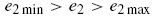
The solution to a complex equation with many numbers of unknowns can be solved by a number of methods. In this paper, a meta- heuristic method and neural network method are used to solve the equation. Particle Swarm Optimization is an intelligent algorithm which mimics the behaviour of birds flocking towards a source of food. The algorithm consists of entities called "particles" which are defined by their co-ordinates in the search space. In our problem, the search space is of five dimensions and each position provides a different value on substituting into the objective function. Meta-heuristic method considers error modelling through error minimization optimization, while neural networks approach trains the neurons to mimic the standard impedance tube. Particle Swarm Optimization is chosen because of its capabilities in solving complex non-linear systems and is used for correcting errors in different applications. In PSO, the particles move according to their velocities to different positions in the search space. Due to their movement, the position co-ordinates are altered and the fitness value of each particle changes. This happens in an iterative process. These velocities are updated (Fig. 3) in every iteration according to the mathematical Eq. (13).
 (13)
(13)
where V new is the velocity of the particle in the current iteration, V old is the velocity of the particle in the previous iteration, c 1 , c 2 and w are tunable parameters, LB is local best solution of the particle and GB is the global best solution of the entire swarm. The localbest is the best solution obtained by an individual particle throughout the iterations. The globalbest is the best solution obtained yet by the algorithm. From the above equation it is observed that the particles move towards better solutions in a swarming nature. As the particles move in the search space, new solutions are obtained. For every new solution, the fitness value of the solution is found in order to determine if the new solution is better or worse compared to the previous solutions. The fitness function is derived from Eq. (12) as
 (14)
(14)
where N is the total number of sample data and i is the sample number. Also the input variables are constrained in the penta-dimensional search space as given in Eqs. (15)-(19).
 (15)
(15)
 (16)
(16)
 (17)
(17)
 (18)
(18)
 (19)
(19)
At the end of all iterations, the global best solution is obtained which is used for compensating the error. The steps for the process are as follows
STEP 1: The following parameters are initialized for optimization
(i) Search space dimension
(ii) Number of particles
(iii) Maximum and minimum limits
(iv) Maximum number of iterations
STEP 2: The particles are distributed randomly within the search space
STEP 3: The fitness value for all the particles are found using the fitness function
STEP 4: The local best and global best values are found from the initial solution
STEP 5: In each iteration,
(i) The velocity of the particles is updated using Eq. (13)
(ii) The new positions of the particles is found
(iii) The new positions are checked for adherence to the constraints
(iv) The fitness value of the new position is found using fitness function as in Eq. (14)
(v) The local best solution for every particle and the global best solution of the entire swarm are updated
(vi) STEP 6: After completion of all the iterations, the global best solution is obtained and is considered for error compensation model.
PSO has several simulation parameters which will define the movement of the particles through the search space. Hence the ideal parameters for optimization should be found by repeated optimization with different simulation parameters.
5.2. Neural network based error corrector
Artificial Neural networks (ANN) consist of groups of entities called neurons which mimic the operations of a biological neuron. These artificial neurons are interconnected and they possess the ability to learn and recognize patterns. Their activity is similar to the human brain. A trained ANN can recognize patterns that are too complex for humans and other computer techniques. The trained ANN can provide results to "what if" scenarios and predict results when sufficient information is provided for analysis. In the brain, knowledge is acquired by forming new interconnections between the neurons. Every new memory triggers a new connection in the brain. The stronger the connection, the better the memory. Usually the connection strength is improved by repeated training. In the same way, the artificial neurons are interconnected in a complex network and the network is altered with new experiences. ANN consists of number of layers of individual neurons. The neurons in a single layer communicate with the neurons in the neighbouring layers. The number of layers also determines the extent of learning of the network. More layers will facilitate more robust network but it slows down the learning process. New learning's are stored as weighting factor in the connections. These weighting factors are corrected through a technique called back propagation which is a feedback mechanism. The pattern recognition ability if the ANN differs with the type of neural network and feedback mechanism. Several classes of neural networks are considered for our problem.
5.2.1. Feed forward network (FFN)
This is the simplest type of ANN where the information flows in only one direction, and there are not any loops in the network, as shown in Figure 4. The first layer is called as the input layer because it receives the input values and the last layer is called the output layer because it provides the results of the neural network. The layers in the middle are called hidden layers, because they represent the internal states of the network and are concealed from the inputs and outputs. Each neuron connection is initialized by a random weight which affect the data flowing across the neurons. The weights are adjusted in a feedback mechanism in an iterative process called back propagation. The iterative process continues until sufficient accuracy is reached.

5.2.2. Radial basis function network (RBFN)
Radial Basis Function networks are similar to FFN expect that they have a radial basis function for activation. Activation function determines the output of the neuron, and is determined by a radial basis function. The output of the network is a combination of parameters of the neuron and the input to the neurons. Each neuron has a prototype vector which is compared with the input of the neuron. The radial distance between the two determines the output of the neuron. The value drops exponentially as the distance increases.
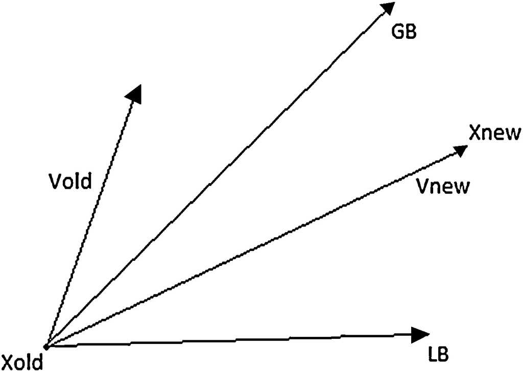
5.2.3. Probabilistic Neural Network (PNN)
A Probabilistic Neural Network is a feed forward neural network which has a statistical algorithm called kernel discriminant analysis and has an additional layer called summation layer in addition to the previous three layers (Fig. 5). PNN shows faster learning when compared with standard FFN and has inherently parallel structure.
The measurement from the designed impedance tube and frequency are fed as the inputs to the network. The performance of the neural network is dependent on the total number of input datasets. The datasets are collected by repeated experiment on the impedance tube with different materials.
5.3. Testing and validation
The simulation parameters chosen for PSO are given in Table 2.
Table 2 Simulation parameters of PSO.
| S. no | Parameter | Value |
|---|---|---|
| 1 | Number of particles | 50 |
| 2 | Number of iterations | 100 |
| 3 | c 1 | 1.5 |
| 4 | c 2 | 2.5 |
| 5 | w | 0.3 |
Since, the method is a stochastic method, there is bound to be minor deviation in the results and runtime. Hence the optimization is repeated for many times with different parameter set and the best value out of these optimizations is considered. The error values after optimization with different values of c 1 , c 2 for input dataset is given below in Table 3.
Table 3 Performance of PSO with input dataset.
| c 1 = 1.5 | c 1 = 1 | c 1 = 3 | |
|---|---|---|---|
| c 2 = 2.5 | c 2 = 3 | c 2 = 1 | |
| Base MSE | 0.009405 | 0.009405 | 0.009405 |
| PSO modelled MSE | 0.008449 | 0.008449 | 0.008451 |
| % Improvement | 10.16 | 10.16 | 10.14 |
| Mean runtime (s) | 4.375 | 4.410 | 4.432 |
The above table shows that the parameter changes only have a very minor change in the performance of the algorithm. This shows the robustness of the algorithm in solving this problem. The optimized values of the error compensating parameters are given in Table 4.
Table 4 PSO optimized solution set.
| Parameter | Value × 10−8 |
|---|---|
| c | −0.1202 |
| d 1 | −0.5415 |
| d 2 | −0.3512 |
| e 1 | −0.2530 |
| e 2 | −0.3218 |
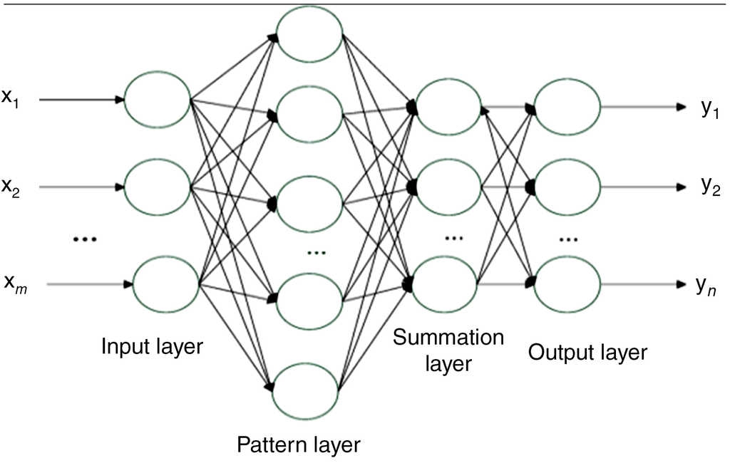
Figure 6 shows the convergence characteristics of PSO attaining an early convergence and its effectiveness in solving the problem. The standard deviation from the best solution is almost none which shows that PSO reaches global minima in almost all the trials.
The solution set given in Table 4 is used to correct the error in the system to a certain extent. In this way the overall accuracy of the impedance tube is improved. The results with a test data is given in Table 5. Here C is the PSO aided error compensated measurement. C is calculated using Eqs. (9) and (12). From Table 5 it is clear that the average error has dropped by nearly 37%. This shows the effectiveness of error compensation technique with a meta-heuristic approach.
Table 5 Test data set for validation with PSO modelled system.
| F (Hz) | Sound absorption coefficient | ||||
|---|---|---|---|---|---|
| Resin felt - 3000 g/m2 and 45 mm | |||||
| B | A | Error A (%) | C | Error C (%) | |
| 80 | 0.048 | 0.045 | 6.25 | 0.0480 | 6.67 |
| 100 | 0.049 | 0.046 | 6.12 | 0.0490 | 6.52 |
| 125 | 0.063 | 0.059 | 6.35 | 0.0629 | 6.61 |
| 160 | 0.093 | 0.091 | 2.15 | 0.0929 | 2.09 |
| 200 | 0.125 | 0.122 | 2.40 | 0.1249 | 2.38 |
| 250 | 0.167 | 0.164 | 1.80 | 0.1668 | 1.71 |
| 315 | 0.229 | 0.222 | 3.06 | 0.2286 | 2.97 |
| 400 | 0.302 | 0.299 | 0.99 | 0.3014 | 0.80 |
| 500 | 0.391 | 0.387 | 1.02 | 0.3901 | 0.80 |
| 630 | 0.509 | 0.505 | 0.79 | 0.5076 | 0.51 |
| 800 | 0.635 | 0.632 | 0.47 | 0.6327 | 1.11 |
| 1000 | 0.775 | 0.762 | 1.68 | 0.7715 | 1.25 |
| 1250 | 0.889 | 0.885 | 0.45 | 0.8835 | 0.17 |
| 1600 | 0.965 | 0.961 | 0.41 | 0.9560 | 0.52 |
| Average error | 2.42 | 2.34 | |||
To test using neural method, the input data set is expanded by making large number of measurements at intermediate frequencies to obtain sufficient training of the neural network. Figure 7 shows the effectiveness of neural network method in error compensation for different number of input dataset.

Neural performance improves with increased input dataset. The neural network is trained with the expanded dataset and the training parameters are chosen as in Table 6.
Table 6 Training parameters for neural networks.
| Parameter | Value |
|---|---|
| Hidden layers | 6 |
| Training ratio | 85 |
| Validation ratio | 10 |
| Test ratio | 5 |
| Training function | Scaled conjugate gradient |
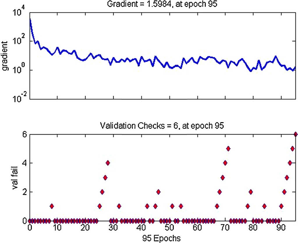
With the above training parameters, the performance of training, validation and testing were observed as 0.168972, 0.11176 and 0.006083 respectively. Figure 8 shows the error histogram and Figure 9 shows the performance of the neural network training while Figure 10 displays the validation of neural network.


With the expanded input dataset, the neural networks modelled error compensation produced an average error of 0.0013 improving the accuracy of the impedance tube by 69.7%. When the trained neural network was used to compensate the errors of the impedance tube with a test dataset, the result was worse compared to the system without error compensation. The test data is tested with the three types of neural network aided error compensator and the results are shown in Table 7. From Table 7 it can be inferred that the system with RBFN neural network has the least error rate when compared to other neural networks. However, neural network has not provided better error correction for the sample under study. It is clear that the average error has increased nearly twice. Hence neural networks require lot of input datasets for effective operation, which is effort consuming.
Table 7 Test data with neural networks modelled error compensation.
| F (Hz) | Sound absorption coefficient | ||||||||
|---|---|---|---|---|---|---|---|---|---|
| Resin felt - 3000 g/m2 and 45 mm | |||||||||
| B | A | Error A | FFN | Error FFN | RBFN | Error RBFN | PNN | Error PNN | |
| 80 | 0.048 | 0.045 | 6.25 | 0.0416 | 7.56 | 0.0482 | 0.42 | 0.0487 | 1.46 |
| 100 | 0.049 | 0.046 | 6.12 | 0.0435 | 5.43 | 0.0545 | 9.18 | 0.0550 | 12.2 |
| 125 | 0.063 | 0.059 | 6.35 | 0.0539 | 8.64 | 0.0586 | 6.98 | 0.0585 | 7.14 |
| 160 | 0.093 | 0.091 | 2.15 | 0.0765 | 15.9 | 0.0826 | 11.1 | 0.0815 | 12.3 |
| 200 | 0.125 | 0.122 | 2.40 | 0.1035 | 15.1 | 0.1081 | 13.5 | 0.1065 | 14.8 |
| 250 | 0.167 | 0.164 | 1.80 | 0.1421 | 13.3 | 0.1758 | 5.27 | 0.1792 | 7.31 |
| 315 | 0.229 | 0.222 | 3.06 | 0.2039 | 8.15 | 0.2165 | 5.46 | 0.2189 | 4.41 |
| 400 | 0.302 | 0.299 | 0.99 | 0.2855 | 4.52 | 0.2940 | 2.65 | 0.2519 | 16.5 |
| 500 | 0.391 | 0.387 | 1.02 | 0.3896 | 0.67 | 0.3284 | 1.79 | 0.3165 | 19.0 |
| 630 | 0.509 | 0.505 | 0.79 | 0.5291 | 4.77 | 0.4999 | 1.79 | 0.5121 | 0.61 |
| 800 | 0.635 | 0.632 | 0.47 | 0.6723 | 6.38 | 0.6151 | 3.13 | 0.6230 | 1.89 |
| 1000 | 0.775 | 0.762 | 1.68 | 0.8200 | 7.61 | 0.7544 | 2.66 | 0.7488 | 3.38 |
| 1250 | 0.889 | 0.885 | 0.45 | 0.9121 | 3.06 | 0.8870 | 0.22 | 0.8991 | 1.14 |
| 1600 | 0.965 | 0.961 | 0.41 | 0.9274 | 3.50 | 0.9942 | 3.03 | 0.9630 | 0.21 |
| Average error | 2.42 | 7.43 | 4.81 | 7.33 | |||||
A comparison of PSO and different neural network modelling reveals that PSO provides good error compensation at all frequencies, while neural network performs only at the mid frequency range. At other frequencies, the error is higher than the original data as evident from Figure 11. Similar experiments were conducted on other materials and the accuracy of the output increased by a significant number, at all frequencies (Table 8). In the table, HL indicates cotton/linen blend aka Halbleinen. With neural network model, the error is reduced for soft felt, whereas increased for other materials, and hence is not a reliable system. PSO modelled system provides better accuracy for all samples and hence is robust and reliable.

Table 8 Output with different test samples.
| F (Hz) | Sound absorption coefficient | ||||||||
|---|---|---|---|---|---|---|---|---|---|
| Glass wool - 800 g/m2 and 40 mm | Soft felt - 40 mm + hard felt - 5 mm | Resin felt - 2000 g/m2 and 30 mm + 2 mm HL | |||||||
| Error without compensator | Error with PSO | Error with RBFN | Error without compensator | Error with PSO | Error with RBFN | Error without compensator | Error with PSO | Error with RBFN | |
| 80 | 04 | 4.00 | 9.05 | 0.3 | 0.29 | 0.66 | 0.3 | 0.30 | 0.08 |
| 100 | 04 | 4.00 | 7.10 | 0.8 | 0.79 | 0.13 | 0.8 | 0.80 | 0.16 |
| 125 | 03 | 2.90 | 2.40 | 0.2 | 0.19 | 0.58 | 0.2 | 0.19 | 0.98 |
| 160 | 04 | 3.90 | 1.80 | 0.2 | 0.19 | 0.57 | 0.2 | 0.19 | 2.14 |
| 200 | 03 | 2.90 | 6.30 | 0.4 | 0.38 | 0.31 | 0.4 | 0.39 | 2.47 |
| 250 | 01 | 0.80 | 9.80 | 5.0 | 4.97 | 2.70 | 5.0 | 4.98 | 2.47 |
| 315 | 03 | 2.70 | 9.20 | 4.0 | 3.96 | 1.18 | 4.0 | 3.96 | 2.57 |
| 400 | 02 | 1.40 | 6.60 | 0.5 | 0.44 | 1.84 | 0.5 | 0.44 | 0.27 |
| 500 | 02 | 1.10 | 1.00 | 1.0 | 0.91 | 1.38 | 1.0 | 0.91 | 0.41 |
| 630 | 13 | 11.6 | 13.6 | 0.9 | 0.76 | 0.20 | 0.9 | 0.76 | 0.75 |
| 800 | 03 | 0.70 | 0.20 | 3.9 | 4.12 | 2.74 | 3.9 | 4.13 | 1.98 |
| 1000 | 03 | 0.50 | 7.70 | 2.0 | 1.64 | 1.80 | 2.0 | 1.65 | 1.32 |
| 1250 | 02 | 3.50 | 3.40 | 4.2 | 4.74 | 1.55 | 4.2 | 4.75 | 5.83 |
| 1600 | 04 | 5.00 | 54.2 | 5.8 | 4.90 | 3.23 | 5.8 | 4.90 | 2.49 |
| Average error | 3.6 | 3.2 | 9.5 | 2 | 1.94 | 1.35 | 2.08 | 2.02 | 2.71 |
Similar tests were conducted with 20 samples and the average mean square error (MSE) obtained for each method is given in Table 9.
6. Conclusion
A mathematical model based error correction system was developed with an intelligent error compensator to minimize errors in a impedance tube. PSO and three types of neural network models namely, feed forward, RBFN and PNN were used to test the system with different test samples. PSO fared well in terms of reduction in error at all frequencies, while neural network based systems reduced the error only at limited frequency ranges. This is attributed to the large training dataset required for neural network. Of the three types of neural network models, RBFN provided better error correction compared to other two models. With PSO, error compensation up to 37% was achieved. The proposed system does not include any additional component or calibration mechanism and thus is a low cost solution. The performance and precision of the impedance tube with intelligent error corrector is similar compared to commercial B&K tubes.

