


 nova página do texto(beta)
 Inglês (pdf)
 Artigo em XML
 Referências do artigo
 Enviar este artigo por email
 Citado por SciELO
  Similares em
SciELO
Similares em
SciELO 
 Permalink
1. Introduction
In the last few decades there has been a dramatic upsurge in the laying of submarine cables and pipelines that are deployed mainly for communications or energy-transfer purposes. Such laying inevitably implies a number of environmental changes which warrant the conduct of environment impact assessment (EIA) studies. Moreover, pipelines are normally deployed at great depths, beyond safe SCUBA diving limits. Remotely operated vehicles (ROVs) are used to collect baseline data as well as to monitor the environmental changes. Whilst unaided human analysis of such video footage allows one to infer qualitative conclusions about the seabed type being studied, the conduction of quantitative assessments through manual means is virtually impossible and highly subjective.
In order to ensure a higher degree of security in energy supply, in 2013 the Maltese government reached an agreement with the Italian government to connect the islands with the European electrical grid. This involved the laying of two 95 km-long submarine electrical cables between Qalet Marku in Malta and Marina di Ragusa in Sicily. As shown by Borg, Lanfranco, Mifsud, Rizzo, and Schembri (1999), Dimech, Borg, and Schembri (2004), Sciberras et al. (2009), and Agnesi et al. (2009), the planned transect intersected with maerl assemblages, which consist of accumulations of calcareous rhodophyte thalli belonging mainly to Corallinaceae and marginally to Peyssonneliaceae (Fig. 1).

In this study, the applicability of various Machine Learning (ML) techniques for the automatic classification of the seabed into maerl and sand regions from recorded ROV footage, was investigated. The developed prototype contributes by providing an alternative or to supplement costly and highly labor-intensive acoustic benthic mapping techniques. The manual analyses of collected video footage is also elevated and a non-subjective approach to quantify the seabed type is made available.
Examples of artificial intelligence (AI) methods used for seabed classification can be found in literature; however, most studies consider acoustic backscatter data. Stephens and Diesing (2014) used multi-beam echo-sounder data collected from the North Sea to classify the substrate types. In this case, the ground truth was determined through the collected samples. Moškon, Žibert, and Kavšek (2015) also demonstrated how classifiers can be applied to raw multi-beam acoustic data for seabed mapping. Similar studies were carried out by Coiras and Williams (2009) and Landmark, Solberg, Austeng, and Hansen (2014). Investigations of seabed classification from image data were not found. As suggested by Stephens and Diesing (2014), reliable automated approaches that provide quantitative results and which can be included in monitoring programs are still relatively novel. While backscattered acoustic signals highlight the differences in the seabed clearly, surveys making use of such signals require a lot of planning, a lengthy permitting procedure, and are very expensive to run. In this study, camera footage captured by an ROV is used. The required data can also be recorded by a towed down-facing camera and is independent of the water transparency and of differences in the lightning conditions.
The following section provides further details on the video footage and how the frames were extracted. Details about the classification methods used and the obtained results are discussed in Sections 3 and 4, respectively. Planned future work and concluding remarks are given in Section 5.
2. Image data
For this study, 2 h and 24 min of video footage which were recorded by the down-facing camera of the ROV over five seabed stretches of 500 m were processed (Fig. 2). The ROV transects followed the path proposed for the submarine interconnector cable. The RAW video was captured at 29 frames per second and recorded on digital media in MPEG2 format. The processing was carried out on frames of 720 × 480 pixels. Since the velocity of the ship was kept constant during data capture, the coordinates of each frame could be computed from the corresponding timestamps. In Table 1, the starting and ending coordinates (in decimal degrees), the average depth, the average vessel speed and the number of frames extracted for every stretch are summarized.
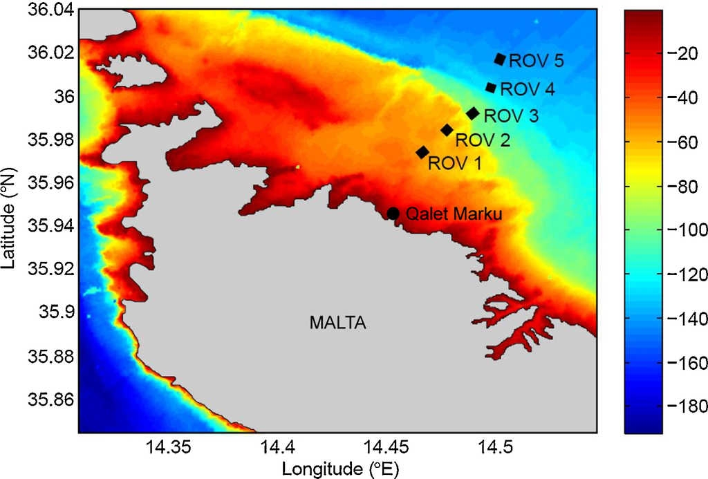
Fig. 2 Bathymetry close to the Maltese islands and the five seabed stretches of 500m (total of 2.5km), staggered through 1000m-long intervals, over which ROV footage was recorded.
Table 1 Average depth, average vessel speed and number of frames extracted for every ROV stretch.
| ROV | Starting coordinates | Stopping coordinates | Average depth (m) | Average vessel speed (m/s) |
Number of extracted frames |
|---|---|---|---|---|---|
| 1 | 35.972830° N, 14.465499° E | 35.976048° N, 14.469327° E | 53.10 | 0.2462 | 33 |
| 2 | 35.982762° N, 14.476914° E | 35.986069° N, 14.480641° E | 60.40 | 0.3910 | 99 |
| 3 | 35.990776° N, 14.489086° E | 35.994190° N, 14.492703° E | 96.84 | 0.2811 | 100 |
| 4 | 36.002065° N, 14.498090° E | 36.006408° N, 14.499593° E | 96.84 | 0.3098 | 100 |
| 5 | 36.015201° N, 14.502245° E | 36.019428° N, 14.504150° E | 138.07 | 0.3038 | 99 |
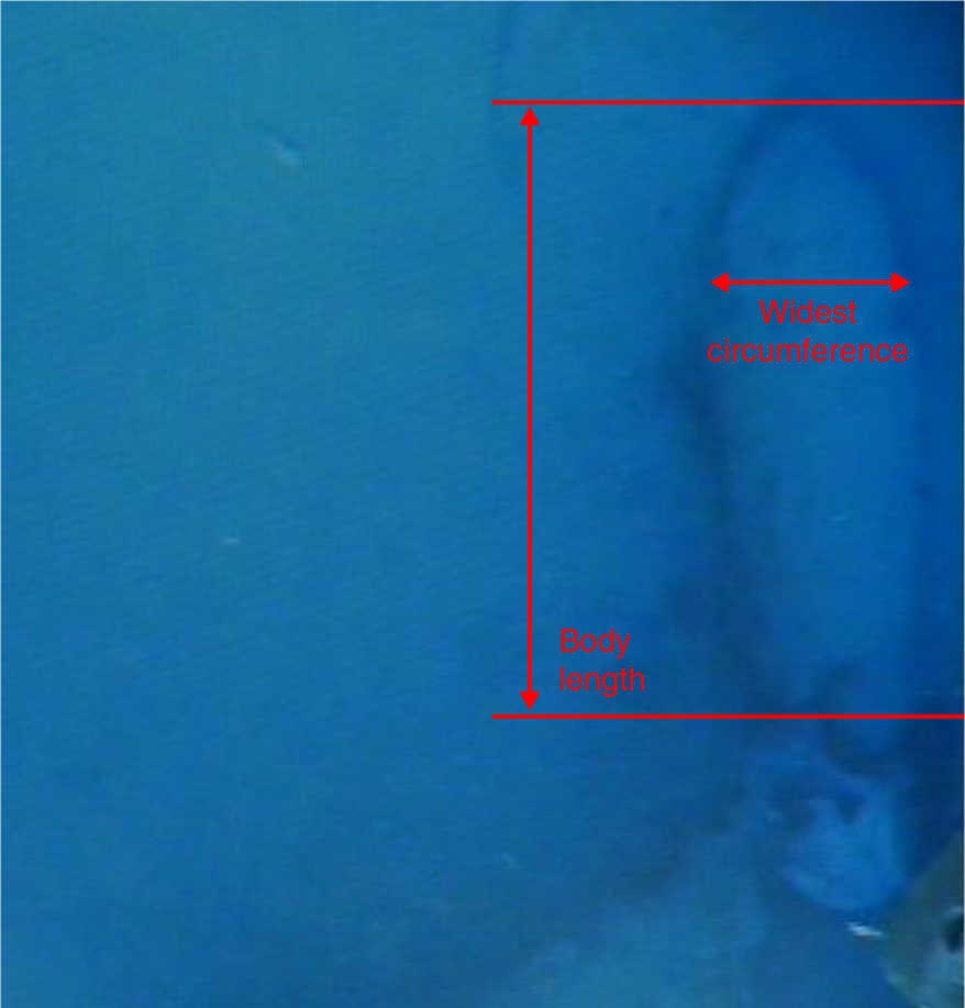
The resolution of the raster set was estimated with frames that showed artifacts of known dimensions. In particular, reference was made to a bomb shell dating from World War II which was captured in a number of frames (Fig. 3). As documented in Boyd (2009), the body length (from the tip without the tail fins) and the diameter at the widest part of such 500-lb general purpose bombs are of 90.67 cm and 30.02 cm, respectively. The number of pixels representing these lengths were obtained from five different frames and the averages were found to be 301.84 and 92.87 pixels. By using these two measurements, an estimate for the physical dimension of individual pixels could be calculated as being 0.003004 m and 0.003233 m, with an average of 0.003118 m. Since the frames consisted of 720 × 480 pixels, each scene represented an area of 2.2451 m × 1.4968 m.
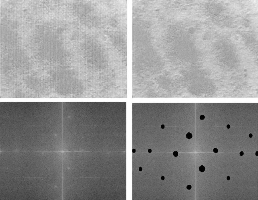
Some of the frames were found to contain periodic noise that contaminated the signal. Such frames were projected onto the Fourier domain and any high frequency components away from the central axes were masked out to remove this periodic pattern. Figure 4 depicts the noise removal process on the blue channel in both the image and Fourier spaces. Through this enhancement, no extra information or artifacts was added to the image data and the luminous values remained unchanged.
3. Feature extraction and classification methods
The task of seabed classifying is a typical classification problem in which samples or pixels are to be categorized into groups. The main objective of this study was to investigate which model most accurately predicts whether a pixel belongs to a maerl or sand patch. All classification methods were tested using tuples storing RGB or LAB information to verify whether the classification performance increases when representing the data in different color spaces. Tuples encoding RGB data stored three numbers that ranged from 0 to 255 and which represented the red, the green and the blue intensities of each pixel. When data was projected onto the LAB model, the L channel represented the luminance, the A channel showed the variation from green to red, while the B channel showed the variation from blue to yellow. Typical training examples and the corresponding values are shown in Figure 5.

Fig. 5 Training sample representations in RGB and CieLAB spaces together with the corresponding class number and the color.
Decision tree learning is based on the pioneering work done by Hunt in the late 1950s. Early in the 1960s, Quinlan developed the Iterative Dichottomizer 3 (ID3). This was followed by the improved C4.5 decision tree learners (Kohavi & Quinlan, 2002). In this work, the J48 method (an implementation of the C4.5 algorithm), the CART (Classification and Regression Tree) and Random Forests (with 10 as well as 50 trees) methods, were tested. Such classification schemes sort samples by determining the corresponding leaf node after traversing down the data structure from the root. Most of the available methods construct the tree by adopting a greedy search strategy and use an information gain evaluation function to determine whether or not an attribute can represent the training samples. Branches of the tree are built by recursively repeating this process for each node and the process stops when all elements in the subset at a point have the same value as the target variable, or when splitting no longer adds value to the predictions (Mitchell, 1997). The constructed tree can be then used as a rule set for predicting the category of an unknown sample from the same set of attributes.
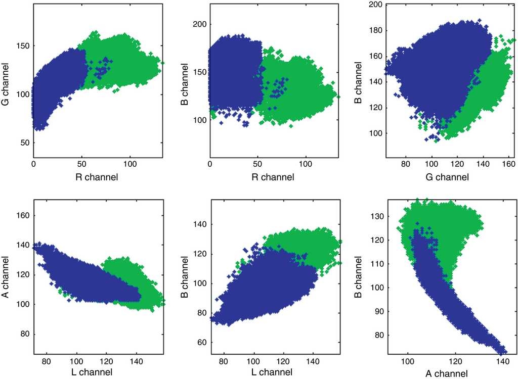
In this study, the applicability of an artificial neural network (ANN) for the classification of data in maerl and sand pixels, was also investigated. Such a learning model connects a number of neurons that take a set of inputs and produce a single real number. The learning algorithm determines numerical weights to apply between each of these elements to obtain the desired output. An advantage of this technique is that it can produce good results even when the input is noisy or incomplete. In particular, a backward propagation network with a 3:7:1 structure was constructed. In Figure 6, combinations of RGB and LAB channels are visualized to highlight natural separation of the two classes. These graphs show that even in two dimensions, the data is separable and hence the neural network model was expected to be able to accurately learn how to differentiate between sand and maerl pixels.
4. Results and model performance
The performance of each model was tested on separate data sets for each individual ROV stretch, as well as on a combined and randomized global set. Classification was carried out on RGB and LAB spaces. The labeled data was manually created by importing the frames in Adobe Photoshop and painting over maerl and sand patches by solid green and solid blue colors, respectively. The created masks were then imported in Matlab to extract the class information (Fig. 7).
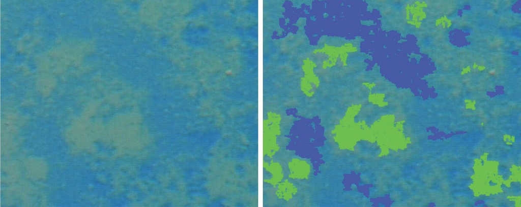
Fig. 7 Original frame from which training values are extracted (left) and the manually generated mask to highlight the pixel locations to be used for training and the corresponding taxonomy class (right).
Testing was performed on labeled data using 10 fold cross-validation. In each experiment, the data was divided into ten groups and the algorithms were run for ten times. At every iteration, nine groups were used for training while the remaining group was used to test the performance of the model. Such a methodology ensured that each training sample was used for testing at least once.
The resulting confusion matrices that show the number of correctly and incorrectly classified samples for all tested methods, are presented in Figure 8. In Figure 9, the actual percentage accuracies which represent the ratio between the sum of true positives and true negatives are listed together with the total number of samples processed. Following the classification of every pixel, an estimation of the total benthic area covered was determined. The results for the first three ROV stretches are presented in Table 2.
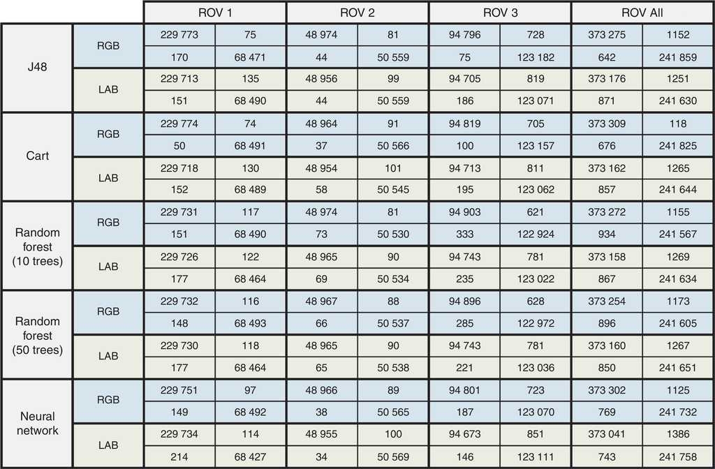
Fig. 8 Confusion matrices for all runs performed. Each 2×2 grid shows the true positive, false negative, false positive and true negative in row major order.
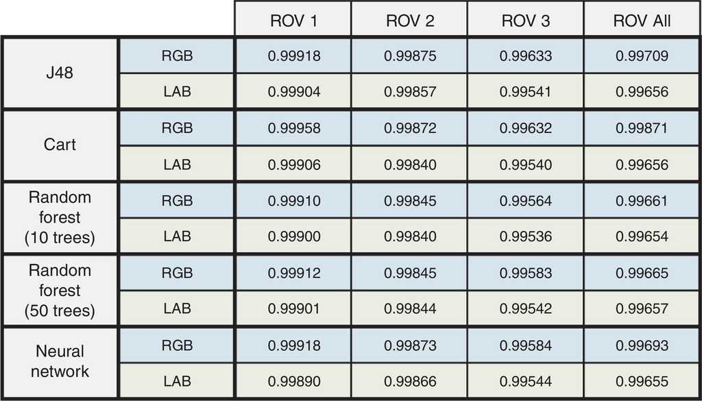
Table 2 Results for the first three ROV stretches.
| ROV 1 | ROV 2 | ROV 3 | |
|---|---|---|---|
| Number of valid frames | 32 | 99 | 6 |
| Total number of pixels processed | 9,574,400 | 29,478,339 | 1,786,566 |
| Pixels classified as sand | 5,493,067 (57.37%) | 10,314,343 (34.99%) | 876,397 (49.05%) |
| Pixels classified as maerl | 4,081,333 (42.63%) | 19,163,996 (65.01%) | 910,169 (50.95%) |
| Estimated total surface area coverage (m2) | 93.0816 | 286.5862 | 17.5000 |
| Estimated sand surface area coverage (m2) | 53.4032 | 100.2753 | 8.5203 |
| Estimated maerl surface area coverage (m2) | 39.6784 | 186.3000 | 8.8000 |
In this study, all ML algorithms produced good results. For half of the tested cases, the J48 algorithm produced the best results. The CART method gave the best performance in the remaining cases. While good results were also achieved by Random Forest with 10 trees, significantly better accuracies were not recorded when using 50 trees. The additional time and memory required to carry out such runs is not worth the small (×10−5) increase in percentage accuracy. The same applies for predictions made with the ANN method.
The J48 and CART methods constructed a representative decision tree in a few seconds. The generated data structure could be easily parsed to provide an accurate output in a very short time. Such techniques can only be used when the output class is discretized; nevertheless, most real value systems can be adapted to work with data bins that range over a very small interval, allowing for these classification methods to be utilized.
In this study, experts in seabed morphology classification were involved at all the stages so as to ensure that the model outputs made sense and agree with what is expected in the real world. Such techniques can easily be applied by other scientists working in other fields of research, such as terrestrial vegetation classification or in the generation of cloud cover masks.
5. Conclusion
This work investigated various Machine Learning techniques for automated seabed classification into maerl and sand patches. The very good and promising results that were obtained suggest that the proposed methods can be used as an alternative or to supplement more costly or more labor-intensive acoustic benthic mapping techniques which include multibeam sonar and side-scan sonar. The laborious and time-consuming manual analyses of collected video footage or still images of the seabed is also elevated.
As summarized in the study for NOAA (Finkbeiner, Stevenson, & Seaman, 2001), imagery and remote sensing methodologies are becoming frequently used for the identification of benthic assemblages. Whilst manual examination of video footage and still images of maerl assemblages is common in the literature such as in Hinz et al. (2010), very few studies, if any, have ever proposed an automated image analysis protocol for ROV footage in order to determine benthic percentage cover of maerl. Expert manual examination of ROV footage has the benefits of enhanced taxonomic resolution over automated examination of the same material and allows for taxonomic identification down to a much lower taxonomic rank. Identification of different maerl bed types is even possible; nonetheless, manual techniques are time-intensive, require taxonomic expert input and can only provide approximate quantitative measures of seabed cover of different benthic assemblages for comparative purposes. Both manual and automated techniques should be accompanied by ground truthing and calibration through sample collection from the field for ex-situ examination, and this routine procedure could not be conducted in the present study in view of the prohibitive sea depths involved.
Apart from noise reduction and the binary classification of pixels, this work also investigated the possibility of computing estimates for surface area coverage in square meters. This was made possible by means of detected debris with known physical dimensions as a scale.
While the results prove that very good classification results can be achieved, the quoted area estimates for maerl and sand heavily rely on the validity of the assumption that the ROV was kept at a constant height above the sea bed. Calibration for pixel dimensions was only performed from a few frames in which debris was spotted and the viewing conditions might have varied even across footage of the same ROV stretch. Although footage was across stretches of 500 m and the sea floor topology in the area being studied goes down gradually, keeping the ROV at a constant altitude is very difficult. Future studies should involve a more advanced and modern equipment that is capable of automatically flying at a constant height above the seafloor.
Disparity from the constant speed assumption can only introduce errors in the computed coordinates of the extracted frames. Such a problem can easily be elevated by frequently recording the timestamp of the ROV footage with the corresponding GPS position. In this work, only the time and position of the starting and stopping locations were recorded.
The developed models can be trained on footage captured by any sensor and in any lighting conditions. Comparison of footage recorded by the down facing and front facing cameras is not straight forward because of differences in the mounting angles and fields of view. Direct matching is difficult because the maerl patches attain slightly different shapes. Although this research focused on the classification of just two taxonomy classes, planned future work includes the extraction of texture information to allow for more detailed studies and categorizations.

