


 text new page (beta)
 English (pdf)
 Article in xml format
 Article references
 Send this article by e-mail
 Cited by SciELO
  Similars in
SciELO
Similars in
SciELO 
 Permalink
1. Introduction
In computer graphics literature, a graphical object is mainly defined by two fundamental characteristics: shape which refers to the geometry of the object, and attributes which is more related to intrinsic properties like color or texture (Gomes, Costa, Darsa, & Velho, 1996). Depending on the type of graphical object, one of these characteristics become more dominant, for example in digital images a description of attributes takes more relevance, while in geometric solids a shape representation is the imperative characteristic. Moreover, this difference is also observed in the kind of mathematical model used to represent such characteristic. While discrete models are preferred to image description, functional representations are typically used in geometric and solid modeling. However, due to grayscale images present the properties of a monochrome function (Velho, Frery, & Gomes, 2009), in this paper, this type of images emerge as the more suitable kind of graphical object with the capability of joining the two fundamental graphical characteristics through a continuous functional model, preserving not only a good approximation of the object geometry but also a precise description of graphical attributes. In our proposal, the color attribute (set of luminance or pixel intensity values) is used to construct a two-dimensional function which defines the height of the graph at each coordinate in the image spatial domain. At this point, the challenge consists in obtaining a suitable continuous function from the set of discrete pixel values. In this regard, it is important to clarify that the numerical technique of fitting input sparse data points by a mathematical function is not a novel strategy used in graphical objects, in fact it can be found in a variety of visualization applications like image processing (Amat, Donat, Liandrat, & Trillo, 2006; Biancardi, Lombardi, & Pacaccio, 1997; Gao, Zhang, Zhang, & Zhou, 2008; Scharinger, 1997;), computer graphics (Feng, Nishita, Jin, & Peng, 2002; Mukundan, 2012), pattern recognition (Oden, Ercil, & Buke, 2003; Subrahmonia, Cooper, & Keren, 1996; Tashk, Helfroush, & Dehghani, 2010; Tarel & Cooper, 2000), and computer-aided geometric design (Heine & Berger, 2012; Park, 2001), among others. For example, in Wu, Wang, and Chiu (2015) a spline interpolation is proposed to image up-scaling with the aim of improving resolution and sharpness, in Ho and Zeng, (2012) a bi-cubic regression is used to achieve better resolution and reduction in border zigzag effects, in Zhang, Chan, Zhang, et al. (2009) a local polynomial regression is applied to high-resolution image reconstruction, and Zhang, Chan, and Zhu (2009) presents a method for image restoration by using least-squares in polynomial regression. Nevertheless, it is important to emphasize that in all of these cases, the interpolated function is always obtained with the main purpose of processing data instead of using it as a proper representation model. In contrast, in this paper, our particular interest is to explore the viability of using continuous interpolated functions as an alternative model description of grayscale images, furthermore, its possible application to image processing is also considered. In relation to this, it must be highlighted that although there are in literature many function estimation methods based on polynomial regressions and spline approximations, our interest centers on the so-called piecewise-linear approach which in recent references (Jiménez-Fernández, Cerecedo-Nuñez, Vazquez-Leal, Beltran-Parrazal, & Filobello-Nino, 2014; Jiménez-Fernández, Vazquez-Leal, et al., 2014), has been successfully used to represent two-dimensional image curves, specifically devoted to laser projection. Moreover, in Jiménez-Fernández, Cerecedo-Nuñez, et al. (2014) a comparative study exhibited a better curve fitting performance of piecewise-linear in comparison to their spline and polynomial counterparts. Among the most emblematic piecewise-linear models reported in literature (Chua & Deng, 1986, 1988; Chua & Kang, 1977; Guzelis & Goknar, 1991; Kahlert & Chua, 1990; Van Bokhoven, 1998), the simplicial representation of Pedro-Julian (Julian, Desages, & Agamennoni, 1999) is taken as reference in our exploratory study. The main reasons for adopting this model are: its superior performance due to its capability to represent n -dimensional functions, and the direct programmability of the function construction methodology which is widely reported in literature (Julian, Desages, & Agamennoni, 1998; Julián, Desages, & D'Amico, 2000; Julián, 2003). The content of this paper is organized as follows. In Section 2, the basic idea of the use of continuous piecewise-linear functions to represent grayscale images is exposed. Section 3 is devoted to describe the piecewise-linear simplicial algorithm for constructing a continuous two-dimensional function. Examples and discussions about the experiment results of the proposed approach are given in Section 4. Finally, conclusions are drawn in Section 5.
2. Basic idea
Let it consider a grayscale image I constituted by (n × m) representative components of brightness-level, I i, j , for i = {1, 2, ..., m}, and j = {1, 2, ..., n}.
In a traditional image representation model, these components are picture elements (pixels) that can be considered as sampling values defined in a rectangular spatial grid data X 1 X2 . Under such approach, an image perception depends on how each point in space associates a color level to that point. However, if the pixel sampling values are linear interpolated around each (i , j)-th coordinate with the aim to construct a continuous piecewise-linear function F (X 1 , X 2 ) = I, then the resulting F ( X ) = I can be used as an alternative representation model. Basically, this model maps the rectangular set of gray levels into a continuous function whose geometric graph depicts the image itself, namely, it means a mathematical recasting from a discrete model to a continuous one. In order to clarify terms, this concept is graphically illustrated in Fig. 1.
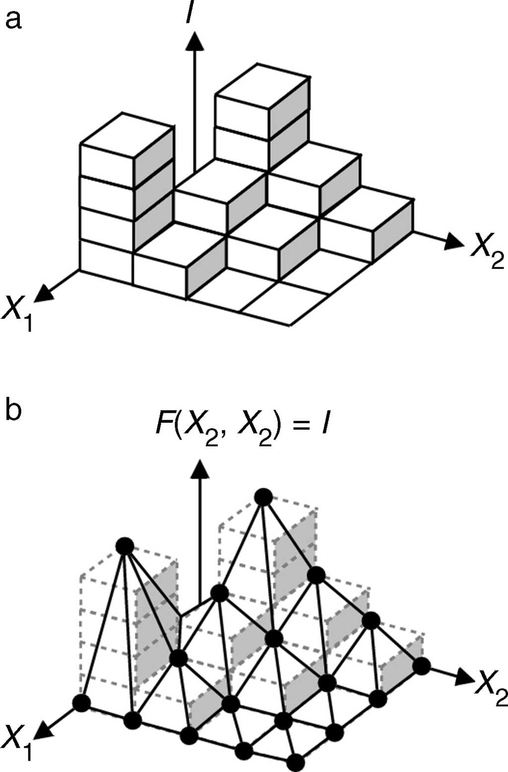
Fig. 1 Grayscale image representation. (a) Discrete pixel array. (b) Continous piecewise-linear function.
Under this alternative representation, a better performance can be obtained in the way the image is visually perceived. Although a more detailed analysis of this point is given in Section 4, it is relevant here to notice, the immediate improvement that can be achieved in resolution and visual acuity. It means, compared with the traditional array representation, an image enhancement is directly obtained from the countinous functional model due to additional sub-graylevels are incorporated into the function.
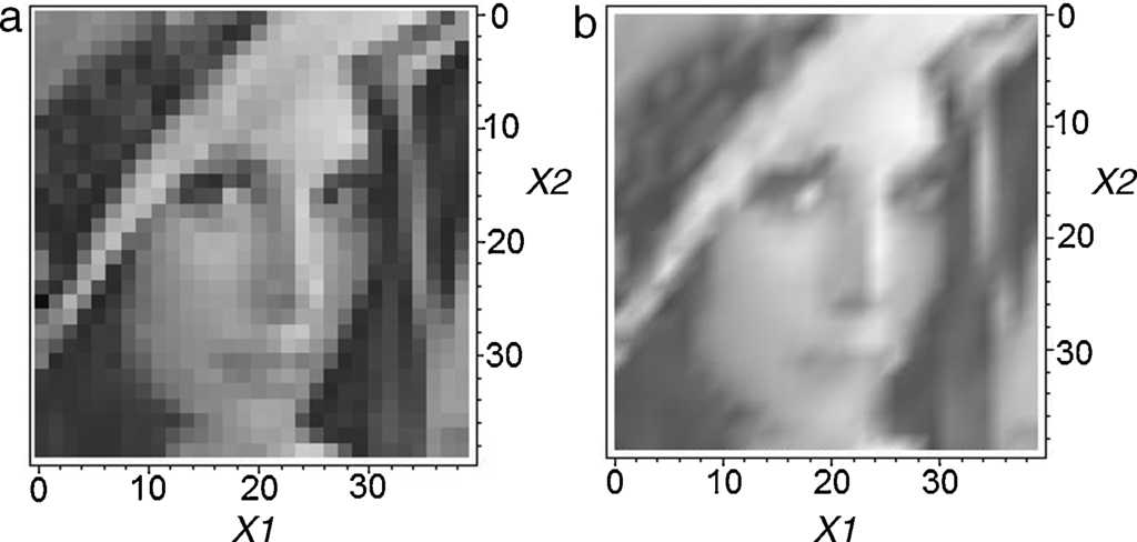
This effect is more evident in low resolution images. To illustrate this, it should be consider the examples of the visual comparisons shown in Fig. 2 and Fig. 3, respectively.
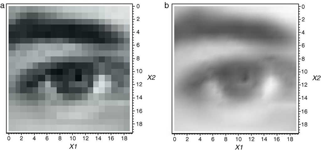
Fig. 2 (20×20)-resolution grayscale image. (a) In a pixel format. (b) In a piecewise-linear functional format.
3. Function construction algorithm
Based on the simplicial piecewise-linear methodology of (Julian, 1999), our proposal for the construction of the continuous function F ( X ) = I is summarized as follows.
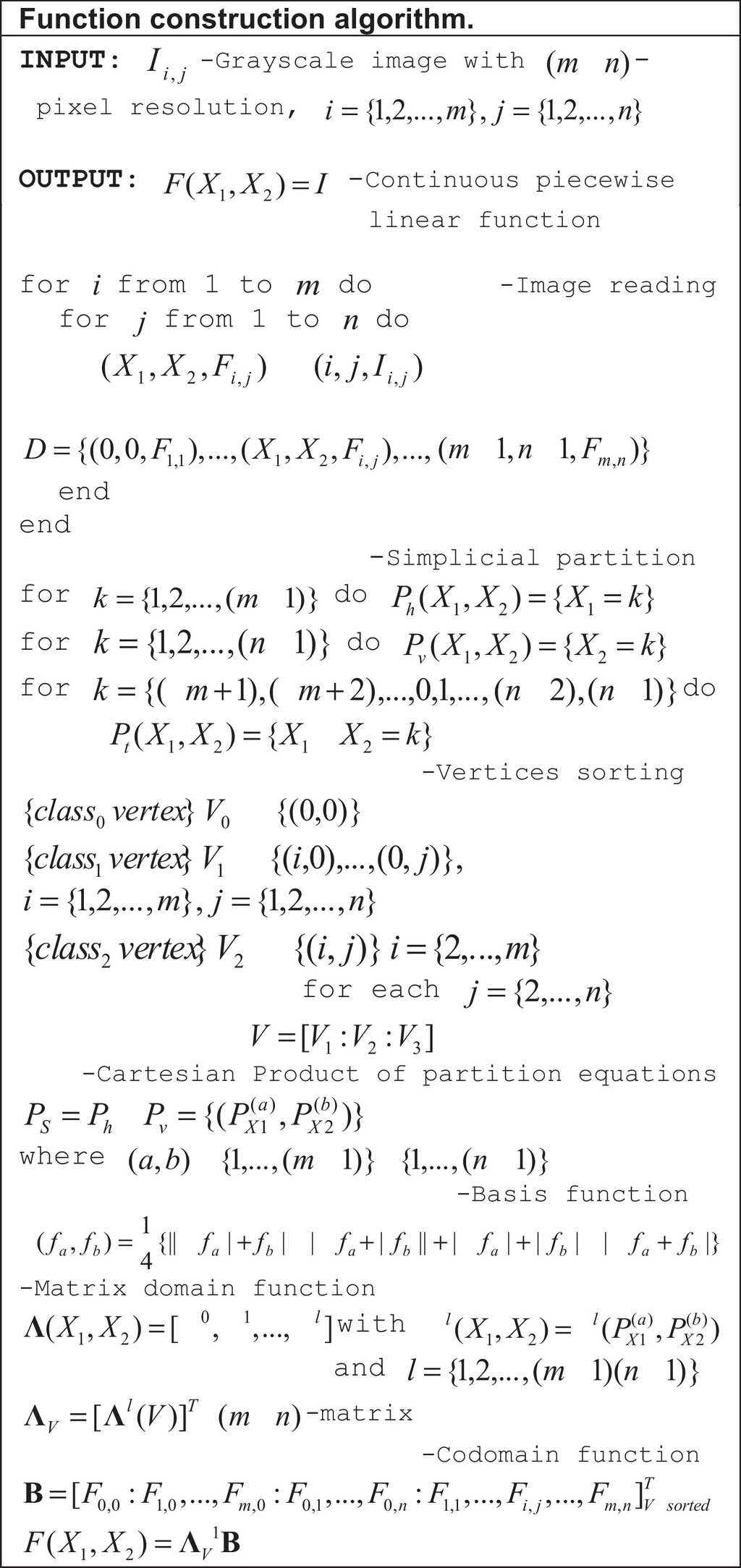
This algorithm is divided into seven consecutive numerical steps: Image reading, Simplicial partition, Vertices sorting, Symbolic basis-function generation, Basis function evaluation, and Codomain and interpolated function construction.
3.1. Image reading
In this step, every image value I i, j is read from the pixel matrix array, and then it is collected and associated to its matrix position in order to form the data structure
D = {(0, 0, F 1,1 ), ..., (X 1 , X 2 , Fi, j ), ..., (m − 1, n − 1, Fm, n )} .
3.2. Simplicial partition
The (i , j)-th matrix position is mapped to its corresponding spatial coordinate in a function domain X 1 X 2 . From a geometric perspective, such function domain is considered as a linear {X 1 X 2 } -plane; moreover, the discrete spatial coordinates can be seen as the breakpoints of an arbitrary continuous piecewise-linear function F (X 1 , X 2 ). In accordance with the interpolation methodology of Pedro-Julian, the function domain must be equally sized partitioned into triangular blocks denoted simplices. The simplicial partition of the domain is done by line equations which are directed to three types of traces: horizontal (Ph (X 1 , X 2 ) = X 1 = k), vertical (Pv(X1,X2)=X2=k), and transversal (Pt (X 1 , X 2 ) = X 1 − X 2 = k). Particularly, for each of these traces the sweep of k must be done in accordance with the boundaries existing along to the X 1 and X 2 axis. For example, if the restrictions X 1 = m and X 2 = m are given, then three k -sweeps : k = 1, 2, ..., (m − 1), k = 1, 2, ..., (n − 1), and k = (−m + 1), (−m + 2)..., 0, 1, ..., (n − 2), (n − 1) will correspond to the vertical, horizontal, and transversal traces, respectively.
3.3. Vertices sorting
The vertices (piecewise-linear function breakpoints) must be ordered according to their class in the vector V = [V 1 : V 2 : V 3 ]. For the domain X 1 X 2 , the class-zero vertex (V 0 ) is the point (0, 0) which is located at the origin of the coordinate system, the class-one vertices (V 1 ) are the coordinates (i , 0) and (0, j) (for i = {1, 2, ..., m} and j = {1, 2, ..., n} , respectively), and the set of class-two vertices (V 2 ) is constituted by the coordinates (i , j) with the j -th index running as j = 1, 2, , m, for each i -th value from 1 to n.
3.4. Symbolic basis-functions generation
In the simplicial partition of X 1 X2 -domain will be a set of (m − 1) horizontal line equations (Ph (X 1 X 2 )), and a set of (n − 1) vertical line equations (Pv(X1X2)). If a cartesian product PS=Ph×Pv between these two sets is formed, then each ordered pair (whose first component is an equation member of Ph and whose second component is an equation member of Pv) is evaluated to form the basis-function vector Λl(X1,X2 )=[ Λ0,Λ1,...,Λl ] with Λ(X1,X2),=γl(P(a) X1 ,P(b) X2), for l = {1, 2, ..., (m − 1)(n − 1)}, and γ (·) defined as γ(fa,fb )=1/4{||−fa |+fb |−|−fa +|fb ||+|−fa |+|fb |−|−fa +fb |}
3.5. Basis-functions evaluation
The vector Λ is evaluated at each ordered vertex. It is important to observe the similarity that exists between the methodology that is used to order vertices and that used to construct the matrix Λ V which is constituted by the rows of evaluated vectors Λl (V). That is
 (1)
(1)
where r indicates the number of vertices denoted as r = (m − 1) × (n − 1).
3.6. Codomain and interpolated function construction
Two operations are involved in this step, in the first one the values of function at the breakpoint coordinates are provided by following a sorted order associated with the vertices {V 0 , V 1 , ..., V r }. These values are collected in vector B and written as follows
 (2)
(2)
Finally, in the second one, the mathematical operation F(X1,X2) = Λ −1 V B is performed.
4. Experiments and discussion
This section explores, by means of illustrative examples, the processing capability of the alternative image representation model. Specifically, two characteristics are examined: the sharpness that is itself present in the image as a result of being described by a continuous function, and the contrast that is obtained by applying functional filters. Additional to these experiments, the potential usage of the model in image analysis techniques such as volume computation is also discussed.
4.1. Sharpness
In regards to sharpness, although the level of clarity of details in images is usually analyzed by considering two fundamental factors: the edge contrast defined as acutance, and the amount of information within the image denoted as resolution, in our comparative discussion only acutance is approached, this because resolution is a factor more closely related to the number of pixels per spatial dimensions. This fact, definitely restricts its application to only pixel image based representations. As reference, let it consider the pixel and function interpolated images shown in Fig. 6.
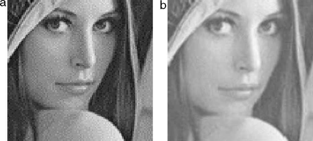
Fig. 6 (100×100) grayscale image: (a) in a traditional pixel format and (b) in a piecewise-linear function interpolated format.
Taking into account that acutance describes how quickly image information transitions at an edge, from the above figure, it can be seen that while in the pixel format (Fig. 6(a)) a remarkable edge transition can be noted, in the function interpolated format (Fig. 6(b)) a smoothing edge transition is observed. From this observation, it is possible to conclude that in Fig. 6(b) a lower acutance is present. In this sense, it is important to notice that although it could be considered preferable to have a high acutance (because it let to obtain sharper and more detailed borders), in low resolution images it is not the best option. This effect is more notorious in three image details of Fig. 6: in the hat, in the cheek, and in the shoulder, where it can be seen that besides to look like less noisy, Fig. 6(b) also shows smoothing traces that contrast with the squared or zigzag traces of Fig. 6(a).
4.2. Contrast
Contrast defines the level of separation between the darkest and brightest areas. A high contrast image exhibits a full range of tones, from black to white, with dark shadows and bright highlights. A low contrast image, exhibits a poor difference between its lights and darks areas what results in a flat appearance. In order to illustrates the viability of modifying contrast in images described by a function interpolated representation, Fig. 7 shows the results obtained in the reference image after applying an exponential functional filter. At this point it is important to clarify that the concept of functional filter has been introduced to describe a mathematical operation that is applied to the continuous interpolated image representation. It has been denoted here as functional to remark the difference with the common mask filters used the traditional pixel representation format of images.
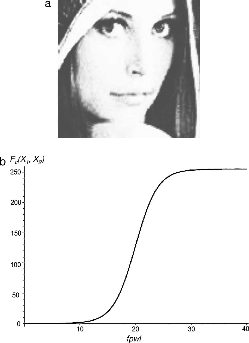
Fig. 7 Results obtained from contrast experiments in the (100×100) grayscale interpolated function image of reference: (a) image with modified contrast and (b) characteristic curve of the functional filter.
In order to simplify nomenclature, let it be the notation F(X1,X2) =fpwl, where F (X 1 , X 2 ) is the piecewise-linear function that represent the reference image depicted in Fig. 6. In the experiment of contrast variation, the functional filter whose result and characteristic curve are shown in Fig. 7, is given by the mapping formulation
 (3)
(3)
where Fc (X 1 , X 2 ) is used to denote the continuous function which represents the modified contrast image of Fig. 7(a).
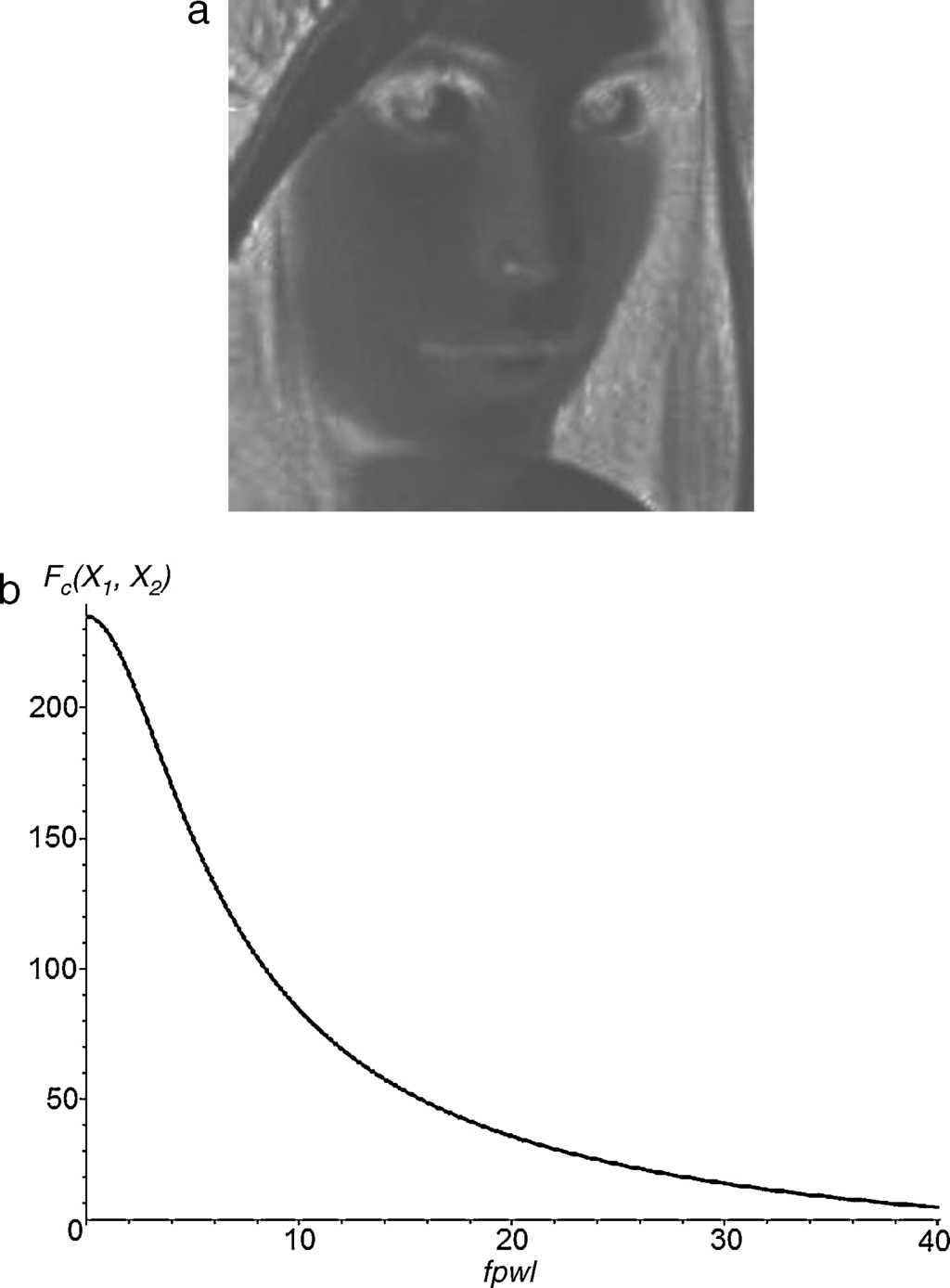
Additional experiments results of contrast variation are provided in Fig. 8 and Fig. 9, where the corresponding functional filters used to obtain such visual effects are Eq. (4) and Eq. (5), respectively.
 (4)
(4)
 (5)
(5)
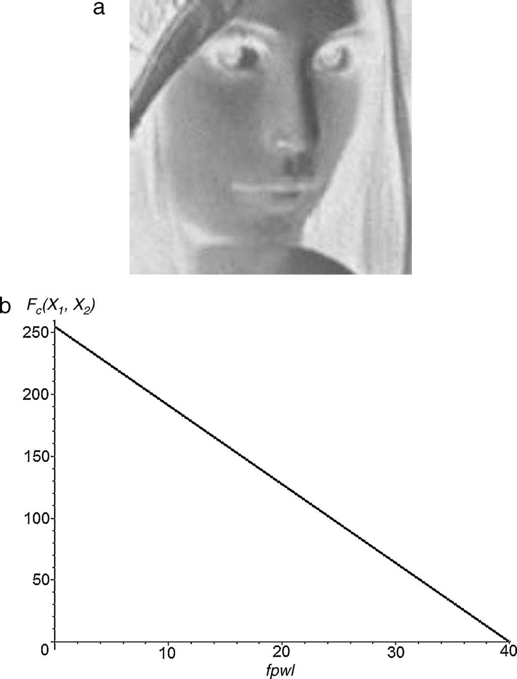
Fig. 8 Additional results obtained from contrast experiments in the (100×100) grayscale interpolated function image of reference: (a) image with modified contrast and (b) characteristic curve of the functional filter.
4.3. Volume estimation
The last experiment, here reported, is related to volume estimation by image processing. In that regard, it is important to mention that dealing with an image representation based on a continuous function exhibits a direct advantage in comparison with the conventional pixel model. On the one hand, it must be observed that due to F (X 1 , X 2 ) = I is an explicit expression, then from a purely mathematical point of view, the approximated volume estimation can be computed as
 (6)
(6)
where the integrand ranges: [ X(i)1, X(f) 1] and [ X(i)2, X(f)2], define the selected surface (function domain), and δ corresponds to the scale factor which must be included in order to denormalize the computed volume results. On the other hand, if a traditional pixel strategy is used to volume estimation, firstly, a tridimensional object compound of two-dimensional contours acquired from segments slices must be constructed, and secondly, the approximated volume must be calculated by adding each consecutive slice surface. From a numerical point of view, under the traditional discrete strategy, the volume computation results from a summation procedure, where every three-dimensional pixel (usually named as voxel) is added on a regular grid space. In order to explore the potential application of the alternative image representation in volume estimation, the microsphere of Fig. 10 is considered.
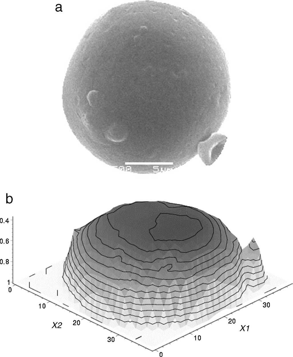
Fig. 10 Microsphere image of reference: (a) original grayscale image and (b) top geometry view of the scaled image to (40×40) resolution.
In our experiment, the algorithm stated in Section 3 was implemented in Maple Software version 15 to construct the piecewise-linear function F (X 1 , X2 ) = I of the (40 × 40) grayscale image of Fig. 10(b). After that, Eq. (6) was used to compute its volume, resulting a normalized (δ = 10) value of 276.141761 cubic units, when the numerical method of Monte-Carlo is applied with a tolerance constraint of 0.5 × 10⁻¹⁴.
5. Conclusion
In this paper the viability of using a continuous two-dimensional piecewise-linear function to describe an arbitrary grayscale image was explored. The function construction methodology of Pedro-Julian was used as reference model to fit the set of discrete graylevel values in a simplicial piecewise-linear geometric surface. The plot of the resulting function showed the possibility of sketching not only the image shape but also incorporating additional attributes like gray level color. Experiments in low-resolution images showed that piecewise-linear functions are a valid alternative model for image representation. Besides of the evident improvement in the visual perception that results from mapping a discrete pixel scheme into a continuous plot, a smoothing transition can also be observed in consecutive high-contrast gray levels. This natural property let it perceive a better resolution and a reduction in border zigzag effects. Finally, it must be highlighted that the alternative representation scheme also exhibited compatibility with image processing operations, particularly, successfully results were obtained by applying functional filters for image-contrast as well as for computing three-dimensional volume estimation.

