


 text new page (beta)
 English (pdf)
 Article in xml format
 Article references
 Send this article by e-mail
 Cited by SciELO
  Similars in
SciELO
Similars in
SciELO 
 Permalink
1. Introduction
Laboratory and commercial ovens are used in a broad variety of applications, from cooking to industrial processing (Mullinger & Jenkings, 2008). By considering their energy source they can be broadly classified into two groups, fuel-based and electric ovens (Mullinger & Jenkings, 2008; Trinks, Mawhinney, Shannon, Reed, & Garvey, 2004). Electric resistance heating has various advantages over systems based on fuel combustion, such as increased control accuracy and heating speed. Thus, electrical heating constitutes a suitable choice for developing laboratory instruments, especially those demanding small heating volumes and precise temperature control (Corona, Maldonado, & Oliva, 2007; Devaraju, Suresha, Ramani Radhakrishnam, 2011; Gam, 1996; Merlone, Iacomini, Tiziani, & Marcarino, 2007). As a general rule, laboratory ovens must operate at established temperatures and avoid temperatures that may damage the samples or their components. Uniform temperature at prescribed zones is also a frequently desired feature, which may be difficult to achieve. All these requirements demand a rational mechanical design, thermodynamic (mathematical) simulations, and the implementation of a suitable control system (Mullinger & Jenkings, 2008). At the industrial level, the majority of the feedback controllers comprise a form of proportional-integral-derivative (PID) loop, mainly because of its simplicity and the vast literature available on PIDs (Johnson & Moradi, 2005; Ogata, 2010). Analog PID controllers work through pneumatic, electronic, electrical or combinations thereof, although with the use of microprocessors, digital versions have been created for these controllers (Ogata, 2010). The major advantages of digital systems are the flexibility and decision making features. The availability of inexpensive digital computers and the benefit of working with digital signals have promoted the current trend towards digital control systems (Ogata, 1995). During the design processes, thermodynamic modeling may assist in the design of the oven (Abraham & Sparrow, 2004; Mistry, Ganapathi, Dey, Bishnoi, & Castillo, 2006). Modeling may assist in the selection of appropriate dimensions and design parameters, saving important amount of resources which would be otherwise wasted in expensive trial and error. Besides simpler analytical efforts (Abraham & Sparrow, 2004), numerical models such as those based on the finite element method have allowed the study of rather complex systems (Depree et al., 2010; Mistry et al., 2006; Najib, Abdullah, Khor, & Saad, 2015; Ploteau, Nicolas, & Glouannec, 2012). Nevertheless, a numerical approach is often very particular for the oven in question, and thus difficult to utilize as a general design guide. Another way to approach the simulation of ovens is the use of the lumped parameter method, which consists in a simplification of the system of equations as a network of discrete elements with reduced number of nodes (Ramallo-González, Eames, & Coley, 2013; Ramirez-Laboreo, Sagues, & Llorente, 2016; Underwood, 2014); although this method reduces the computational time, a set of appropriated parameters should be known to calibrate the model.
Given this background, this work aims to develop and characterize an electric laboratory oven to achieve uniform temperatures for studying small (1 cm × 1 cm) polymer nanocomposite samples heated below 300 °C, by controlling the heating temperature with a minimum precision of 0.3 °C by means of a PID control. Thermodynamic balance renders a set of differential equations that are used to predict the temperature evolution in the major components of the oven. As an application example, the oven is used to provide uniform, precise and controlled heating to small carbon nanotube/polymer composites, for their use as thermoresistive sensors. The design approach used here, the governing differential equations proposed and the characterization methods employed may assist other researchers and engineers in the design of dedicated, low temperature, high precision controlled ovens.
2. Oven design
2.1. Mechanical design
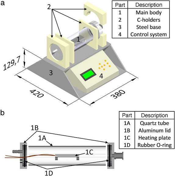
The main body of the oven consists of a 300 mm long quartz tube with 80 mm outer diameter and 2.5 mm wall thickness. The quartz tube has two solid aluminum lids made of 102 mm diameter circular plates. The oven is supported by a trapezoid-shaped steel base, which encloses the control system. A couple of internal supports for the body of the oven and C-shaped holders for fixing the tube and lids were manufactured from Nylamid plates, see Figure 1 a. C-holders at the end of the body of the oven hinge into two sections to allow the removal of the lids. Ceramic fiber-cloth was used to thermally isolate the supports from the oven body. Sealing of the oven is achieved by Viton® O-rings hermetically adjusted between the quartz tube and aluminum lids. The aluminum lids include feedthroughs for electrical wires, which connect the heating element contained inside the quartz tube to the power supply, as well as for thermocouples and wires. K-type thermocouples were used to measure the temperature inside the oven, with the reference one located typically over the heating plate or directly over the sample (depending on the experiment), see Figure 1 b. The aluminum lids also have connectors for potential gas supply, although this feature was not used herein. The heating element was fabricated from a 12.7 mm thick rectangular aluminum plate with in-plane dimensions of 95 mm by 38 mm, containing an electric cartridge heater (electrical resistance) supplied with 120 V AC at a nominal frequency of 60 Hz. The heating plate also contains a small hole which receives a thermocouple for temperature monitoring. The oven lids can be removed to introduce the samples, placing thermocouples or simply to access the heating plate. To prevent samples from sticking to the heating plate, a Teflon-coated fiber glass fabric cover (∼200 μm) was used.
2.2. Electric and control system
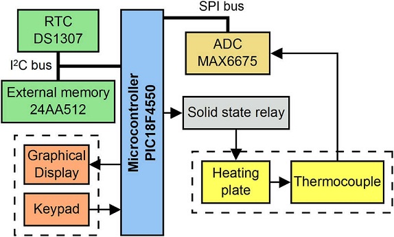
The oven was designed to operate with a power supply of 120 V (AC) at 60 Hz. Electrical current/voltage measurements showed that the mean power demanded by the electrical resistance (cartridge heater) was 60 W. The control system uses a microcontroller implemented on a specially designed electronic board, similar to the control system used in other devices reported in the literature (Affanni, 2013; Ahlers & Ammermuller, 2013; Devaraju et al., 2011; Oliveira, Freire, Deep, & Barros,1998). A schematic of the electronic components and the interconnections of the control system are shown in Figure 2. The microcontroller chosen for the control system is the PIC18F4550 (Microchip Technology, Chandler, USA), mainly because it includes a serial communication module which assists in the interconnection with other integrated circuits via an I2C protocol (Predko, 2008). Other relevant components used are an analog-to-digital converter (ADC) MAX6675 for K-type thermocouples (Maxim Integrated, San Jose, USA), a real time clock (RTC) DS1307 (Maxim Integrated, San Jose, USA), for the sampling time of the controller, and a solid state relay RM1A23D25 (Carlo Gavazzi Inc., Buffalo Grove, USA) used to control the resistance heater. In addition to the components listed above, the system includes a graphical display which shows information about the oven operation and temperature in real time and a keypad that allows the user's interaction and programming.
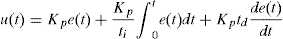
To ensure that the oven keeps the temperatures set by the user with minimal oscillations, a PID control routine was developed which periodically supply voltage adjustments to the heater resistance. The continuous control equation of a signal u(n) for a PID controller in time (t ) domain is (Ogata, 2010),
 (1)
(1)
where e (t ) is the error signal, K p is the proportional gain, t i and t d are the integral and derivative time constants, respectively, and the derivative is with respect to time. The instantaneous error e (t ) is computed as the difference between the desired temperature and the actual (measured) temperature.
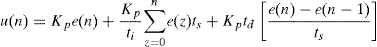
Because of the discrete nature of the control circuit board, a discrete version of the PID controller equation is required, such as (Ibrahim, 2006),
 (2)
(2)
with n a positive integer and e(n) as the n th error sampling and t s the sampling time (instead of a time differential). The PID control signal u (n ) is supplied to the heating element by a pulse width modulation (PWM) signal with a time period denoted by t s .
In order to calibrate the constants and sampling time of the PID controller, the Ziegler and Nichols tuning method (Ziegler & Nichols, 1942) was used. A step voltage was applied to the electrical heater and the response of the heating element to such a stimulus was registered. The Ziegler-Nichols method proposes an approximation of the oven as a first order system with a time delay, using the unknown control constants as:
 (3a)
(3a)
 (3b)
(3b)
 (3c)
(3c)
where τ 0 is the time delay, γ 0 is the time constant and κ 0 is the static gain. τ 0 is defined as the time between voltage application and the onset of temperature rise; γ 0 is the required time to reach 63% of the set temperature, after the time delay has elapsed. Both τ 0 and γ 0 are obtained from the time step response graph. κ 0 indicates the temperature change due to a change in applied voltage and is calculated as the difference between the steady state temperature and the initial temperature divided by the applied voltage. For the sampling time (t s ), it is recommended to choose a value between t s < τ 0 /4 or t s < γ 0 /10.
To implement this method for the control of the oven, the temperature at the center of the heating plate surface was continuously registered by a thermocouple connected to a data acquisition system. The heating element was fed with an input voltage of 24 V AC (∼20% of the supply voltage) by a PWM signal. The PID control routine was programmed in the microcontroller by using a PIC-C compiler which allows complex routines development in relatively short times.
In this case, the Ziegler-Nichols method yielded signal overshooting and was thus used only as a first approximation to calculate the control parameters. Therefore, a second method proposed by Chien, Hrons, and Reswick (1952) was further used for tuning the control variables. These authors suggest using the same step response of the Ziegler-Nichols method but with a new definition of the controller constants as,
 (4a)
(4a)
 (4b)
(4b)
 (4c)
(4c)
2.3. Measurement of the temperature distribution and dynamic profiles
A series of experiments were performed to characterize the thermal behavior of the proposed oven. Those initial experiments did not include samples, since only the oven temperature was of interest during this first stage. The experiments included measurements of the dynamic evolution of temperature at specific locations of the oven, and measurements of the heating plate temperature at different locations of the plate. All temperature measurements were performed by K-type thermocouples within a range of 20-350 °C.
For the first set of experiments, the temperature at three locations of the oven was simultaneously monitored for heating-cooling cycles from 25 °C to 300 °C. The three thermocouples were located at the mid-length of the quartz tube, two at the interior of the tube (T 1 and T 2 ) and the third one at the exterior (T 3 ), as shown in Figure 3 a. The thermocouple T 1 was located at the center of the heating plate, considered as reference for the heating plate, Figure 3 b. Thermocouple T 2 measured the temperature of the inner cavity (air), while thermocouple T3 monitored the temperature of the external surface of the quartz tube, see Figure 3 a. The test comprises a heating phase from 24 °C to 300 °C (in ∼21 min) and immediately the heating source was turned off, allowing natural cooling of the oven. The total period of temperature monitoring was about 2 h.
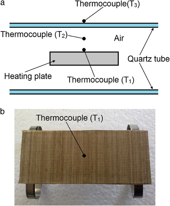
Fig. 3 Location of thermocouples for temperature measurements: (a) inner air (T2) and oven body (T3), (b) heating plate (T1).
To investigate the spatial distribution of temperature on the surface of the heating plate (Fig. 3b), measurements at different locations were conducted in a second experiment. In this experiment, a grid of 15 rectangles of 12.7 mm by 19 mm was drawn on the top surface of the heating plate, and the temperature at the center of each small rectangle was taken as representative of such areas, as shown in Figure 4. This experiment allowed assessing the uniformity in temperature on the heating plate.
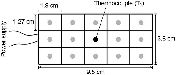
Fig. 4 Locations of temperature measurement on the surface of the heating plate. The dark central point was taken as reference (T1).
In addition to these two tests, temperature measurements were conducted on the contact area between the quartz body and the Nylamid supports, in order to verify that the temperature does not exceed the glass transition temperature of Nylamid.
3. Dynamic heat transfer model
A dynamic thermal model was developed from an energy balance as a design and predictive tool to assess the temperature evolution of the main components of the oven, viz. the heating plate, the air inside the oven, and the oven body (quartz tube).
The model is based on the cross-section model of the oven shown in Figure 5 a, where the three major elements of the oven are sketched: the heating plate (1), the inner cavity (2) and the main body (3). The aluminum lids were not considered in the model since they are far away (∼100 mm) from the heating plate and insulated by O-rings. As will be discussed, measurements conducted showed that the temperature of such aluminum lids raised only a couple of degrees Celsius upon heating to 300 °C, supporting our assumption. The energy supply (Q 0 ) can be estimated by the applied electric power as Q 0 = IV , where I is the current drawn by the heater resistance and V is the voltage supplied. The external environment (labeled "0") is at temperature T 0 , and the temperature of each of the 1, 2, 3 elements are indicated as T 1 , T 2 and T 3 , respectively.
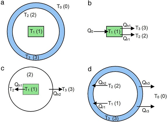
Fig. 5 Cross-section model of the oven considering the three major components and their energy balance: (a) heating plate (1), inner cavity (2) and main body (3), (b) energy balance of element 1, (c) energy balance of element 2, (d) energy balance of element 3.
Assuming that the temperature distribution is uniform at each component (T 1 , T 2 and T 3 ), and neglecting heat losses through the oven lids, an energy balance of each element is performed, see Figure 5 b-d.
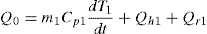
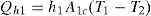
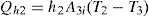
The heating plate (Fig. 5 b) receives a power supply Q 0 and part of this energy is transmitted to the inner cavity of the oven by convection with the internal air (Q h1 ). In most cases, the gas temperature is not affected by radiation, since gases only absorb or emit in narrow wavelength bands, and for this to be significant, it requires considerable large volumes of gas (Çengel, 2003; Holman, 2010). Therefore, it is assumed that the radiated heat (Q r1 ) propagates from the exposed faces of the heating plate to the inner wall of the oven body. Thus, an energy balance of the heating plate yields:
 (5a)
(5a)
The first term on the right hand side of Eq. (5a) represents the energy used to raise the temperature of the heating plate, while the second and third terms represents losses by convection and radiation, respectively; m 1 is the mass of the heating plate and C p1 its specific heat. The convective heat (Q h1 ) can be estimated as (Çengel, 2003):
 (5b)
(5b)
Here, A 1 c is the plate area considered for convection and h 1 is the heat transfer coefficient by free convection of air around the heating plate. According to Holman (2010), h 1 can be estimated by h 1 = 1.32[(T 1 − T 2 )/d eq ]1/4, where d eq is found by approximating the exposed area of the plate (omitting its ends) to the area of a cylinder with the same length and a diameter, such that d eq = 2(b + c )/π , where b = 38 mm is the width of the heating plate and c = 13 mm its thickness.
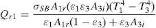
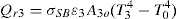
The radiated heat transfer Q r1 is found through an expression for concentric cylinders as (Holman, 2010):
 (5c)
(5c)
where A 1 r and A 3 i are the areas of the heating plate (element #1) and the inner area of the oven body (element #3) which are exposed to radiation, σ SB = 5.67 × 10⁻⁸ W/m2 K4 is the Stefan-Boltzmann constant and ɛ i (i = 1, 2 or 3) is the emissivity of the materials. The subscripts 1 and 3 refer to each element of the system outlined in Figure 5 a.
Substituting the convection, Eq. (5b), and radiation, Eq. (5c), terms into Eq. (5a) leads to the energy balance for the heating plate:
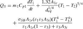 (5d)
(5d)
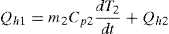
The energy balance of the inner cavity is depicted in Figure 5c. Assuming that the fluid into the oven is air, the convective heat transfer from the heater is Q h1 and the convective heat transfer of the air to the inner wall of the oven body is Q h2 , the energy conservation equation applied to element 2 in Figure 5 c yields:
 (6a)
(6a)
with C p2 as the specific heat of the inner fluid (air) and m 2 its mass.
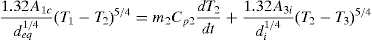
The convective heat transfer Q h2 in Eq. (6a) can be expressed as (Çengel, 2003):
 (6b)
(6b)
where h 2 = 1.32[(T 2 − T 3 )/d i ]1/4 with d i as the inner diameter of the quartz tube (element #3 in Fig. 5a) which has a corresponding inner area A 3 i .
Substituting Eqs. (5b) and (6b) into Eq. (6a) yields:
 (6c)
(6c)
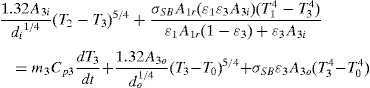
Finally, the energy balance of the oven body (element 3) is shown in Figure 5d. In this condition, the quartz tube receives convective heat from the inner fluid (Q h2 ) and radiation heat from the heating plate (Q r1 ). The oven body (quartz tube) uses part of such energy to raise its temperature, and dissipates part of the energy to the environment by convection (Q h3 ) and radiation (Q r3 ), i.e.:
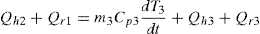 (7a)
(7a)
The process of convection heat transfer to the external environment (Q h3 ) at temperature T 0 , can be expressed as:
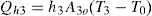
Here, h 3 = 1.32[(T 3 − T 0 )/d o ]1/4 with d o as the external diameter of the quartz tube with a corresponding surface area A 3o , exposed to free convection.
The thermal radiation losses (Q r3 ) can be estimated by Çengel (2003):
 (7c)
(7c)
Substituting Eqs. (5c), (6b), (7b), and (7c) into Eq. (7a) leads to:
 (7c)
(7c)
Defining the constants C i (i = 1-9) as:
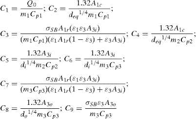 (8a-i)
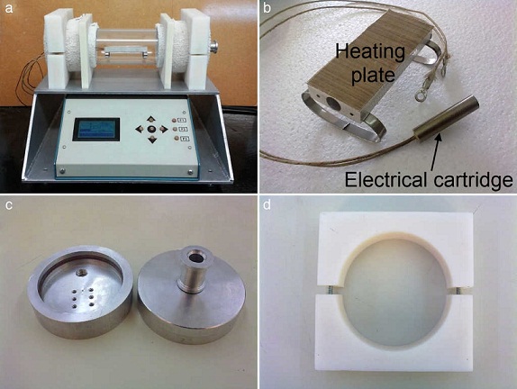
Eqs. (5d), (6c) and (7d) can be rewritten as:
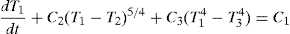 (9a)
(9a)
 (9b)
(9b)
 (9c)
(9c)
Eqs. (9a)-(9c) are the governing differential equations of the thermal problem and correspond to a system of three first order nonlinear coupled differential equations, which are rather complex to solve analytically. The solution of Eq. (9) represents the dynamic evolution of the temperature of each element in Figure 5, i.e., T 1 (t ), T 2 (t ) and T 3 (t ). In order to solve Eqs. (9a)-(9c), a numerical solution was obtained by using the Ruge-Kutta method implemented in MATLAB ®. The initial conditions of the heating problem were considered as T 1 (0) = T 2 (0) = T 3 (0) = T 0 . Cooling right after reaching a maximum temperature (T imax, i = 1, 2, 3) was also considered in a separate simulation. To predict cooling using Eqs. (9a)-(9c), the term corresponding to the heating source was eliminated (C 1 = 0 in Eq. (9a)) and the initial conditions of this second simulation were taken as the final temperatures of the heating problem, i.e., T 1 (0) = T 1 max, T 2 (0) = T 2 max, T 3 (0) = T 3 max .
The material properties and thermal constants used in the simulations were obtained from the literature (Çengel, 2003; Holman, 2010; Incropera, Dewitt, Bergman, Lavine, 2007; Kern, 1965) and are grouped in Table 1.
Table 1 Material properties and thermal constants used in the heat transfer model (Çengel, 2003; Holman, 2010; Incropera et al., 2007; Kern, 1965).
| Property [unit] | Element (symbol) | Value |
|---|---|---|
| Mass [kg] | Heating plate (m 1 ) | 0.14 |
| Internal fluid (m 2 ) | 2.4 × 10⁻³ | |
| Quartz tube (m 3 ) | 0.387 | |
| Specific heat [kJ/kg K] | Heating plate (C p1 ) | 0.9 |
| Air (C p2 ) | 1.0 | |
| Quartz tube (C p3 ) | 0.7 | |
| Emissivity | Heating plate (ɛ1) | 0.4 |
| Quartz tube (ɛ 3 ) | 0.93 | |
| Surface area for radiation/convection [m2] | Heating plate, convection (A 1 c ) | 10.5 × 10⁻³ |
| Heating plate, radiation (A 1 r ) | 9.48 × 10⁻³ | |
| Quartz tube, internal (A 3 i ) | 70.7 × 10⁻³ | |
| Quartz tube, external (A 3 o ) | 75.4 × 10⁻³ | |
| Density of air [kg/m3] | (ρ air ) | 1.77 |
| Diameter used for convection [mm] | Equivalent for heating plate (d eq ) | 3 |
| Quartz tube, internal (d i ) | 75 | |
| Quartz tube, external (d o ) | 80 | |
| Stefan-Boltzmann constant [W/m2 K4] | σ SB | 5.67 × 10⁻⁸ |
| Reference temperature [K] | T 0 | 298 |
| Heater power [W] | Q 0 | 60 |
The input power (Q 0 = 60 W) was found by measuring the electrical resistance (257 Ω) and current (483 mA) flowing through the heater using an Agilent U1252A digital multimeter. The mass of the air in Eq. (6a) (m 2 ) was obtained by the product of its density (ρ air = 1.77 kg/m3) and the volume of the inner cavity (v int ). For the heating plate, the area considered as exposed to convection (A 1 c ) was the entire surface of the heating plate, while for radiation the area exposed (A 1 r ) omits the edge surfaces of the heating plate. For the oven body, A 3 i and A 3 o correspond to the internal and external faces of the quartz tube, respectively, and both surfaces were used to calculate heat transfer by convection and radiation.
4. Thermoresistive materials characterization
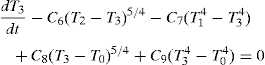
Once the oven was constructed and thermally characterized, it was employed for characterizing the thermoresistive behavior of small samples of polymer composites based on carbon nanotubes. The thermoresistive samples were fabricated by solution casting, using a high temperature engineering thermoplastic polysulfone (PSF) and commercial multiwall carbon nanotubes (MWCNTs). PSF was acquired from Solvay Advanced Polymers (Alpharetta, USA) and MWCNTs were supplied by C-Nano Technology (San Francisco, USA). The nanotubes have inner diameters of 4-6 nm, outer diameters of 17-19 nm and lengths around 1-2 μm. MWCNT/PSF composites in thin film geometry were fabricated at 0.3 wt.% by using the solution casting method (Bautista-Quijano, Avilés, Aguilar, & Tapia 2010), which produced MWCNT/PSF wafers of ∼86 mm diameter and ∼200 μm thickness, Figure 6a. Specimens for thermoresistive characterization were obtained by cutting a 1 cm square section from the wafer and subsequently bonding copper wires with silver paint for electrical resistance measurements, as seen in Figure 6 b.
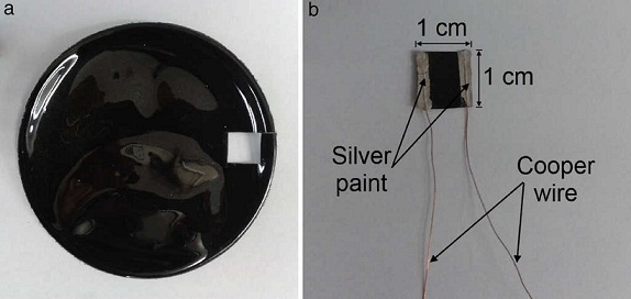
Fig. 6 MWCNT/PSF composites for thermoresistive characterization using the constructed oven: (a) as-produced MWCNT/PSF wafer, (b) final specimen.
The MWCNT/PSF specimens were centered on the heating plate and a thermocouple was placed on top of the specimen to measure its temperature. Simultaneously, a digital multimeter with data login capabilities (Agilent U1252A) was connected to the terminals of the specimen to measure its electrical resistance in situ while the sample was heated/cooled. During heating, the oven was configured to generate a 5 °C/min ramp from room temperature (∼25 °C) until a maximum temperature of 100 °C was reached. The cooling phase was performed freely. For statistical confidence, three MWCNT/PSF specimens were used as test replicates.
5. Results and discussion
5.1. Oven construction and thermal characterization
5.1.1. Mechanical design
The oven was designed and constructed based on the specifications of materials and dimensions presented in Section 2.1. A photograph of the oven assembly is presented in Figure 7 a. The heating plate and the commercial electric cartridge used as heater source (located inside the heating plate cavity) are shown in Figure 7 b. The aluminum lids which seal the ends of the oven body are shown in Figure 7 c, while a Nylamid holder is shown in Figure 7 d.
5.1.2. Tuning of the PID controller
The calculation of the control parameters was conducted in three sequential steps. In a first step, the Ziegler-Nichols method (Ziegler & Nichols, 1942) was used to provide a first approximation of the control parameters required by Eq. (2). Following this method, the control parameters obtained for a sampling time t s = 1 s were K p = 8.41 V/°C, t i = 62 s and t d = 15.5 s, see Eq. (3). During initial tests using these control parameters, it was found that the obtained calibration generate overshoots of up to ∼20% of the desired signal (see Fig. 8), and a second method for the PID tuning was required. The second method used was the one proposed by Chien et al. (1952) and the control parameters found according to Eq. (4) for a sampling time of t s = 1 s were K p = 4.2 V/°C, t i = 929 s and t d = 15.5 s. By employing these adjusted parameters, the undesired overshoots in temperature were significantly reduced; however, the speed of temperature stabilization was too slow (>10 min). The oscillating overshooting may be attributed to windup or saturation of the controller, caused by a large contribution of the integral term of the control (Ibrahim, 2006; Johnson & Moradi, 2005). In order to avoid this issue, additional fine-tunings were performed to accurately adjust the control parameters. This third and final step regarding the fine-tuning of control parameters was conducted iteratively by using the MATLAB® Simulink tool, where the model of the oven PID controller was simulated. Through this numerical approach, the steady state error and overshooting were minimized with the fastest signal stabilization. The parameters of the PID control obtained by the three different methods are listed in Table 2.
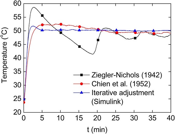
Fig. 8 Effect of the control parameters for different PID tunings. The targeted temperature is 50°C.
Table 2 PID parameters calculated using three sequential methods.
| Method | PID parameter | ||
|---|---|---|---|
| K p (V/°C) | t i(s) | t d(s) | |
| Ziegler and Nichols (1942) | 8.41 | 62 | 15.5 |
| Chien et al. (1952) | 4.2 | 929 | 15.5 |
| Iterative adjustments (MATLAB-Simulink) | 6.5 | 1084 | 2.0 |
As an example of the outcomes of the three methods discussed, Figure 8 shows an experiment where a step function of 50 °C was aimed. As seen from this figure, the Ziegler and Nichols (1942) method yields significant overshoots near t = 2.5 min, which slowly decrease thereafter. The Chien et al. method (Chien et al., 1952) greatly reduces those overshoots, but it demands more than 25 min to stabilize the temperature. The best performance is achieved by setting the control parameters to those found iteratively by the "Simulink" MATLAB® tool, which reaches temperature stabilization in about 5 min.
According to these results, the parameters determined by the iterative calibration method were chosen as the final control parameters. With this settings, the error in the steady state temperature is about 0.6% (0.3 °C), which is close to the minimum temperature variation that the control system is able to record because of the resolution of the ADC MAX6675 (Maxim Integrated, San Jose, USA) used for the thermocouple (± 0.25 °C). Several other tests of the control system, such as heating ramps (not shown), were also satisfactorily conducted. All the tests conducted indicated that the proposed PID controller performance is satisfactory for the oven requirements.
5.1.3. Thermal characterization
The numerical solution of Eqs. (9a)-(9c) is presented in Figure 9 for a heating-cooling experiment lasting 2 h, composed of 20 min heating followed by 100 min of free cooling. According to the simulation, after heating for 20 min the heating plate reaches a maximum (theoretical) temperature of T 1 = 319 °C, while the temperature of the air inside the oven is T 2 = 119 °C. The predicted temperature of the quartz tube is significantly lower, T 3 = 68° C, which is below the glass transition temperature of the Nylamid (∼100 °C) chosen for manufacturing the quartz tube holders. Dynamic profiles obtained from measurements are also shown in Figure 9. It can be seen from this figure that, even with the simplifications of the mathematical model, the predictions from the heat transfer model reasonably agree with the measured temperatures. Within ∼20 min, the heating plate reaches a (measured) temperature of ∼300 °C, while the internal air reaches ∼140 °C. These temperatures satisfy the design temperatures of the oven, i.e., the temperatures required for thermoresistive characterization of polymer nanocomposites. The agreement between the measured and predicted temperature of the heating plate is outstanding, since the thermal mass of such element is small and the assumption of spatially uniform temperature seems reasonable for that element. This is not the case for the air inside the oven main body, where a highly uniform temperature (such as that assumed in the model) is not expected for a 300 mm long quartz tube with 75 mm internal diameter. However, even with this limitation, the difference between the measured and predicted temperature of the air inside the oven is only about 18%. The temperature of the aluminum lids raised only ∼2 °C upon heating, confirming that heat losses through such lids are small. Therefore, the analytical model proposed is capable of reproducing the temperature profiles of the oven with reasonable accuracy and thus represent a valuable and economic tool for the design of similar ovens and simulation of their thermal behavior.
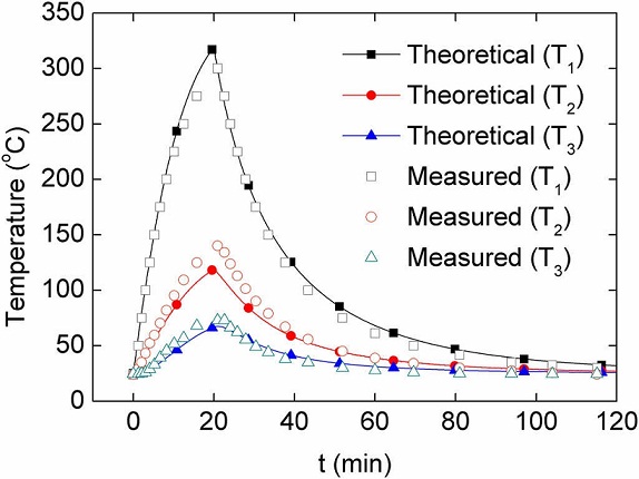
Fig. 9 Measured and simulated temperature of the three major components of the oven during heating and free cooling.
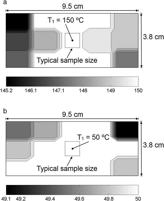
The spatial distribution of temperature on the surface of the 9.5 cm × 3.8 cm heating plate was experimentally investigated. Figure 10 shows contour plots generated from linear interpolations of the temperature measurements conducted on the heating plate as depicted in Figure 4. A reference temperature of 150 °C (at the center of the plate) was chosen to represent the spatial distribution of temperature during the heating phase, Figure 10a, while a reference temperature of 50 °C was chosen for the cooling phase, Figure 10b. For heating and cooling, the temperature distribution is rather uniform (variations are less than 10%) in a 5.7 cm × 3.8 cm zone of the heating plate. Furthermore, the measurements show that within a zone of 3.8 cm × 2.5 cm the temperature variations are less than 0.2 °C. The maximum variations (∼11%) occur at the corners of the plate, and the temperature at such zones should not be considered as representative of the central part of the heating plate. Since the oven was specifically designed for characterization of polymer nanocomposite samples whose typical dimensions do not exceed 1 cm × 1 cm, a homogenous distribution of temperature in the sample is expected to be achieved by using the constructed oven.
5.2. Characterization of the thermoresistive behavior of MWCNT/PSF films
Thermoresistive characterization of the MWCNT/PSF composites described in Section 4 was performed by using the constructed oven. In these tests, samples were placed on the center of the heating plate while a thermocouple and a digital multimeter were used to simultaneously measure the temperature and electric resistance of the sample during a heating/cooling cycle. For heating, the control system was configured to generate a 5 °C/min ramp from room temperature (T 0 ) to 100 °C, while cooling was performed freely.
The initial resistance of the three samples tested (R 0 ) was in the range of 10 kΩ to 20 kΩ. Figure 11 shows the normalized change in electrical resistance (ΔR/R 0 ) as a function of the normalized change in temperature (ΔT/T 0 ) for three replicates. Quite consistent results are observed for the three replicates.
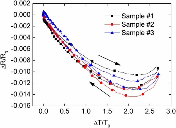
From Figure 11, it can be noted that the electrical resistance of specimens varies with temperature. ΔR/R 0 decreases during heating in a non-linear fashion up to ΔT/T 0 ≈ 2 (T ∼ 80 °C) and the thermoresistive curve settles and then reverses for higher temperatures (2 ≤ ΔT/T 0 ≤ 2.7). The behavior of this material in the range 0 ≤ ΔT/T 0 ≤ 2 resembles the behavior of commercial thermistors with negative thermoresistive coefficient. For these devices, an exponential relationship exists between the decrease in electrical resistance and the temperature rise (Fraden, 2010; Nachtigal, 1990). This preliminary characterization of the thermoresistive polymer composites using the constructed oven shows that the MWCNT/CNT film developed has a potential use as temperature sensor.
6. Conclusions
A dedicated electric oven with PID control specifically designed for the characterization of small (1 cm × 1 cm) thermoresistive polymer nanocomposites was designed, constructed and thermally characterized. The oven is capable of reaching a uniform temperature within ±0.2 °C in an area of 3.8 cm × 2.5 cm, which is satisfactory for the aimed application. Regarding the control system, the presence of temperature overshooting (likely by a windup effect) required tuning the PID control by iterative simulations. The discrete PID algorithm and final calibration parameters implemented are capable of maintaining the temperature of the heating plate with a precision of 0.3 °C. As a design tool, a dynamic thermal model based on thermodynamic energy balance was developed; the model predicts with reasonable accuracy the temporal evolution of temperature at the main elements of the oven, which was probed by comparing the model predictions to measurements. The governing differential equations controlling the thermodynamic performance of the oven deduced here may be of value for the design of other ovens or thermal devices with similar features. Such equations may also further motivate more complex control efforts using, for example, state space controllers. As such, the thermal model constitutes a powerful predictive tool for the design of this and similar ovens, which could save extensive time and resources invested in experiments. As an application example, thermoresistive characterization of carbon nanotube/polymer composites was conducted using the constructed oven; the nanocomposites showed a negative coefficient of thermoresistivity, similar to commercial solid-state semiconductor thermistors.

