nueva página del texto (beta)
 Inglés (pdf)
 Artículo en XML
 Referencias del artículo
 Enviar artículo por email
 Citado por SciELO
  Similares en
SciELO
Similares en
SciELO 
 Permalink
1. Introduction
The economic history of Mexico over the past few decades has shown that exchange rate movements have been highly correlated with the country's inflation rate. The literature about Mexico on this subject has been highly focused on two research topics. The first topic analyzes the non-linearity and magnitude of the pass-through elasticity between the exchange rate and the inflation rate for different periods. For example, according to Capistrán (2012), before 2001 the pass-through between the exchange rate and consumer prices was 0.6%, which indicated that a movement in the exchange parity had a quick effect on prices. The second topic measures the effectiveness of the Mexican Central Bank in reducing the pass-through elasticity implemented in 2001, when a permanent inflation-targeting policy of 3% was announced for the following years. Some examples in the literature covering these two topics are: Frankel et al. (2005), Nogueira (2010), Capistrán et al. (2012), Cortés (2013), Aleem and Lahiani (2013), Peón and Brindis (2014), and Baharumshah, Sirag and Soon (2017).
The pass-through elasticity has been widely analyzed in the literature, at the country level, but such analysis has barely been extended to the regional level, despite the high economic heterogeneity existing between different economic regions in Mexico. Some of the arguments that justify the need to develop new literature focused on measuring pass-through values at a regional level are as follows: First, Mexico’s most important trade partner is the U.S. and the effect of such trade is not homogenous across different geographic regions in the country, as analyzed by Esquivel et al. (2002). Therefore, exchange rate variations would not be expected to have the same effect across different economic regions in the country. Second, the Mexican border region has increased its economic integration with the U.S. economy since the implementation of the North American Trade Agreement in 1994 (now called USMCA). Consequently, since border regions have become more integrated with the U.S. economy (Cortez and Camargo, 2009, Cañas, et al., 2013) border cities are, as expected, more dollarized than others cities in the country and variations in the exchange rate affect the dynamics of prices in those regions differently. If all these arguments are correct, then the monetary policy implemented by the central bank could possibly be creating sub-optimal results at a country level. We believe this topic deserves more attention in the literature. For this reason, the aim of this study is to contribute to filling this gap by proposing an analysis of the potential heterogeneity that could exist between the CPIs of some border and non-border cities.
The contribution of this study is twofold. First, the analysis spans from 2002 to 2019 and includes border and 27 non-border cities. There are few regional studies about Mexico in the literature, but they analyze only the periods before 2010 and not the following years. This article includes in the analysis the years 2011-2019, a period where the Mexican peso depreciated 54% against the U.S. dollar. In addition, the inflation rate reached its highest level in December 2017 since December 2008. Second, the analysis in this study includes a period in which gasoline prices in Mexico were liberalized and raised quickly in the following period. Even though gasoline prices were adjusted through bands with maximum and minimum prices during 20161, the real shock on the inflation rate hit in January 2017, when gasoline prices increased between 16% and 22% in just one month. Therefore, in order to analyze such effect, the analysis has been divided into a period which stops in 2016 and another which includes 2017-2019, the period where gasoline prices started to increase considerably, previous they were liberalized in December 2017. An analysis of this period is deemed relevant because most of the gasoline consumed in Mexico is imported from the U.S. and prices increase in different proportions across the country, reflecting international prices and factors such as exchange rate variations. Moreover, to the best of our knowledge, there is no literature available that captures how the pass-through elasticities varied across places due to this event and how producers and consumers absorbed this shock.
The border cities included in the analysis are Tijuana, Mexicali, Matamoros, Ciudad Juarez, and Ciudad Acuña. They are the only ones included in this study because the National Institute of Statistics and Geography (INEGI) constructs a Consumer Price Index (CPI) just for these border cities in the country. On the other hand, the study includes 27 metropolitan non-border cities2, located across different geographic regions in the country. The analyzed period in the study spans from 2002 to December 2019, with monthly frequency. The study incorporates a VAR econometric model, as well as some impulse response functions which capture how the inflation rate reacted to different shocks in the exchange rate.
The remainder of this paper is organized as follows: Section 2 reviews empirical literature about Mexico related to the exchange rate and inflation rate pass-through effect. Section 3 describes the data, while section 4 addresses the econometric model and justifies the variables used in the study. Section 5 presents the results and some arguments to justify such results. Lastly, section 6 offers the concluding remarks.
2. Review of the Literature on Pass-through in Mexico
In the last fifteen years, most of the literature about Mexico regarding the pass-through between the exchange rate and the inflation rate has been mainly focused on analyzing the effectiveness of the inflation targeting implemented by the central bank of Mexico in 2001. For example, Capistrán et al. (2012) analyze the exchange rate pass-through and different price indices in Mexico. Their results indicate that even though the exchange rate pass-through derived from imported prices is complete, it declines along the production distribution chain; hence, its impact on long-run consumer prices is below 20 percent. Furthermore, the authors mention that Bank of Mexico's adoption of inflation targets has had a significant effect on lowering the price level.
Aleem and Lahiani (2013), using data from 1994 to 2009, consider non-linearities in exchange rate pass-through of domestic prices and estimate a threshold vector autoregressive model. The authors find that domestic prices in Mexico react strongly to a positive one-unit exchange rate shock, just above the threshold level of the inflation rate. Peón and Brindis (2014), in a study from 1980 to 2010, analyze how a change in nominal exchange rate depreciation is transferred to domestic prices. The analysis is carried out using a recursive Structural Vector Autoregression with exogenous variables. Aleem and Lahiani (2013) and Peón and Brindis (2014) also analyze the pass-through effect on prices in the Mexican economy after the Mexican Central Bank implemented an inflation-targeting policy in 2001. Other studies analyzing the effectiveness of the central bank with the inflation-targeting policy are Choudhri and Hakura (2006), Galindo and Ros (2008), Romero and Catalán (2012), Cortés (2013), Baharumshah, Voon, and Wohar (2017), and González and Saucedo (2018).
2.1 Review of the Literature on Regional Pass-through in Mexico
There are few studies in the literature about Mexico which analyze the effect of variations in the exchange rate on regional prices. One of those studies is by Castillo, Varela, and Ocegueda (2013), who analyze the short- and long-run effects of exchange rates on different geographic regions in Mexico, from 1982 to 2007. Results indicate that, in general, pass-through has decreased in the past few years, but results differ across geographic regions for both short- and long-run effects. Similarly, a study by Banxico (2018) finds that pass-through is positive and significant for border cities (0.16% accumulated for 12 months), but has little effect on prices in the rest of the country (the elasticity is around 0.03%), a value that is small in a low inflation rate environment.
Another relevant study is by Solorzano (2017), who analyzes the price history of 85,000 items across 46 urban areas and 58 industries in the country during the period 2002 to 2010. Results indicate that pass-through rates differ across regions and industries. The difference in the pass-through elasticity values between low and high pass-through regions is nearly one third after twelve months. The author indicates that most differences in pass-through rates between regions are explained, among other factors, by demand conditions, economic development, distance to the U.S. border, import intensity, etc. So far, to the best of our knowledge, these are the only two studies available in the literature about regional pass-through in Mexico; this is clear evidence that more studies are needed in this direction.
3. The Data
Capistrán et al. (2012) analyze the pass-through effect of the exchange rate on the inflation rate in Mexico. In the study, they include endogenous and exogenous variables such as: output gap to control for economic activity, interest rate to control for monetary policy activities, industrial production, consumer prices, 3-month Treasury bill rate return (for the U.S.), and international energy commodity prices. In other studies, Romero and Catalán (2012) include the difference between the GDP and the potential GDP (output gap) to control for domestic economic activity. In addition, they control for supply shocks in the United States, such as changes in food and energy prices, which are considered as highly volatile products. In this study, we have included energy prices in the regression estimates.
Table 1 Description of Variables
| Variable Name | Description | Source |
|---|---|---|
| Employment at City Level | IMSS Formal Insured for each city. Proxy for economic development | IMSS Datos Abiertos |
| Cete | 91-day Interest Rate | Monthly data. Banxico |
| Exchange Rate | Currency: Pesos per U.S. dollar | Monthly data. Banxico |
| Country CPI | Consumer Price Index | Monthly data. INEGI, BIE |
| Country Core CPI | Excluding volatile prices, such as food products, energy and government tariffs | Monthly data. INEGI, BIE |
| Acapulco, Aguascalientes, Campeche, Mexico City, Chihuahua, Colima, Cuernavaca, Culiacan, Durango, Guadalajara, Hermosillo, La Paz, Leon, Merida, Monterrey, Morelia, Oaxaca, Puebla, Queretaro, San Luis Potosi, Tampico, Tepic, Tlaxcala, Toluca, Torreon, Veracruz, Villahermosa | Acapulco CPI, Aguascalientes CPI, Campeche CPI, Mexico City CPI, Chihuahua CPI, Colima CPI, Cuernavaca CPI, Culiacan CPI, Durango CPI, Guadalajara CPI, Hermosillo CPI, La Paz CPI, Leon CPI, Merida CPI, Monterrey CPI, Morelia CPI, Oaxaca CPI, Puebla CPI, Queretaro CPI, San Luis Potosi CPI, Tampico CPI, Tepic CPI, Tlaxcala CPI, Toluca CPI, Torreon CPI, Veracruz CPI, Villahermosa CPI | Monthly data. INEGI, Tabulados Índice de Precios |
| Tijuana, Mexicali, Ciudad Juarez, Ciudad Acuña, Matamoros | Tijuana CPI, Mexicali CPI, Ciudad Juarez CPI, Ciudad Acuña CPI, Matamoros CPI | Monthly data. INEGI, Tabulados Índice de Precios |
| U.S. CPI | U.S. Consumer Price Index | Monthly data. Bureau of Labor Stats. (BLS) |
| Energy Commodity Prices | Energy commodity price index | Monthly data. World Bank |
| Service Sector Employment Share | Employment in the service sector in each city/ Total Employment | IMSS |
| Large Firms Employment Share | Emp. in Large Firms/ Total Employment | ENOE, INEGI |
| Gasoline Prices | Gasoline Price Index for 87 and 92 octanes | Monthly data, INEGI, Tabulados |
Source: Authors’ own elaboration.
Some of the variables included in this study are taken from Romero and Catalán (2012) and Capistrán et al. (2012), while others are exclusive to this study since they capture relevant factors from the border and non-border cities. Table 1 displays a description and sources of all the variables included in this econometric model. The variables included in this study are the CPIs for each of the border and non-border cities, the formal employment for each metropolitan area, the interest rate (91-day Cete), the nominal exchange rate, and external control variables such as the U.S. Consumer Price Index, international energy commodities prices, and domestic control variables such as the proportion of people working in the service sector and the proportion of total employees in each city working in large firms (+ 250 employees).
Economic activity could be expected to be different in border cities compared to non-border metropolitan cities. For example, Cañas et al. (2013) mention that the economic integration of Mexican border cities is highly influenced by the economic activity in the U.S. border neighbor cities. As a proxy for measuring the economic labor activity at a city level, the number of employees registered in the formal labor market in each of the cities analyzed in this study has been captured from the Social Security Government Office (IMSS). Such data has been created by gathering employment information from different IMSS delegation offices, a methodology that is considered more appropriate to estimate employment numbers at a city level. This variable can be helpful to control for economic activity in each analyzed city, and, being monthly series, is very useful for this purpose.
Then a service sector employment share variable is constructed. Such variable is the ratio between employment in the service sector (business services, social services, and commerce) in a specific city divided by the total employment in the city. It is estimated because employment in the service sector is expected to be more aligned with the economic activity in such city and less related with the economic activity in external places (i.e. U.S. economic activity). In addition, in order to capture how labor structure changes over time in the analyzed cities, a second variable called (size) is constructed. Such variable is the number of people in a city working in large firms (+ 250 employees) divided by the total employment in the same city. This is relevant because it could be expected that, in general, large firms would be more exposed to trade issues (exchange rate variations) than small firms and, at the same time, some economic sectors would be more exposed to variations in the exchange rate than others.
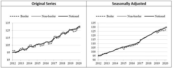
Another variable included in the analysis is the 91-day interest rate (91-day Cete) which captures the monetary policy changes implemented by the Central Bank of Mexico. Such variable is a good measure of changes in the domestic monetary policy in the short-run. The annual percent change in the CPI is another variable included and captures the seasonally adjusted annual inflation rate, as previously done by Capistrán et al. (2012) and González and Saucedo (2018). Section 1.1 in the appendix shows the CPI series before and after the seasonal adjustment.3 The U.S. CPI is included as a control variable because changes in the U.S. consumer prices are expected to be followed by changes in the monetary policy implemented by the Federal Reserve. Lastly, energy prices are also included as a control variable since they reflect global demand expectations, so, ceteris paribus, they must affect the behavior of domestic prices.
The study uses monthly data and spans from January 2002 to December 2019.4 The entire analyzed period is split into two sub-periods. The first sub-period starts in January 2002 and finishes in December 2016, eliminating the potential effects on prices from the gasoline price shocks that began in January 2017. The second period (January 2017 onwards) covers the period in which gasoline prices in Mexico were more volatile.
4. The Econometric Model
This study employs a vector autoregressive model (VAR) to estimate the transmission rate from local currency depreciation to the inflation rate. VAR models allow endogenous and exogenous variables to interact with each other and are useful to construct impulse response functions. The econometric model implemented here is different from those implemented by Capistrán et al. (2012) and Cortés (2013), because it includes external and exogenous exchange rate shocks. The objective in this study is to examine how consumer prices in border and non-border cities respond when there are movements in the exchange rate values. The estimated econometric model examines demand shocks, which, in turn, include changes in employment at the regional level used to control for exchange rate shocks generated by the economic activity. Such models can be useful to identify how each city responds differently to exchange rate shocks.
Before the VAR model is estimated, a Johansen test is implemented to analyze the relationship in the long-run among all the variables. Results indicate that most variables do not show any evidence of cointegration (see appendix section 1.2, a few cities show only one cointegration equation, but most of them none).5 Subsequently, each variable in levels is examined to determine whether or not unit-roots exist. Results in section 1.3 in the appendix indicate that just three variables are stationary in the initial series. To make all of them stationary, the 12th difference of the logarithms is estimated6 and the results are shown in section 1.3 in the appendix. Different unit root tests are implemented, and then the one that reports the best fit is chosen. All unit roots of equations remain inside the unit circle root to obtain stable results. Optimal lags are also reported in table 1.3 in the appendix. Results indicate that all variables, including the CPI for each city, are stationary. Given the previous test results, a VAR model is proposed:
where
4.1 Control Variable Justification
In the VAR model, the U.S. CPI is used as an external shock variable to observe how consumer prices react when prices in the U.S. change. In addition, energy commodity prices are also used as an external variable to observe how the CPI changes after a world price shock. These two variables are exogenous because Mexico is an open, price-taker economy and shocks in the global market affect the formation of domestic prices, but not the other way around. As was already mentioned, a control variable (services) is used and refers to the percentage of people working in the service sector in each of the cities analyzed in the study. A higher percentage is expected to indicate that such economy is less dollarized; therefore, its economic cycle is more dependent on internal factors. In addition, the model controls for firm size values. Such data is obtained from the National Employment Survey (ENOE)8. Shocks in the exchange rate are identified by using generalized impulse response functions9. The central bank could react by modifying the interest rate, which would affect the exchange rate and, consequently, the inflation rate. This mutual dependence among such variables is captured in the econometric model. In addition, the impulse response functions included in this study are like those presented by Koop, Pesaran, and Potter (1996), who defined the generalized impulse response as follows:
The equation (2) measures the effect of one standard error shock in the j
th equation at time t on expected values of x (the vector that included dependent variables in the VAR system) at time t+n. The term
5. Results
This section shows the impulse response functions after developing the VAR model for each of the analyzed border and non-border cities. To see how variations in the exchange rate affect consumer prices, a 1% depreciation in the exchange rate is simulated. Results are presented in elasticities and show the accumulated pass-through effect from variations in the exchange rate to the inflation rate. The elasticity in period ɛ is calculated as follows:
where
5.1 Pass-Through Country Estimates
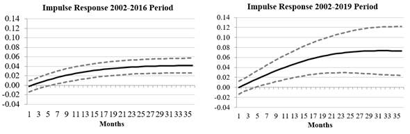
The left-hand graph in figure 1 shows the pass-through elasticity from 2002 to 2016. Those years exclude the 2017-2019 period when gasoline prices increased rapidly. The elasticity value is 0.04% after 36 months. Confidence intervals in figure 1 (in dotted lines) show that zero is excluded, thereby indicating that they are relevant and statistically different from zero.
Note: We recognize gasoline prices were liberalized in December 2017, but prices started to increase considerably since January 2017 and sometimes we refer as if the liberalized price period were started since January 2017.
Source: Author´s estimations using data from ENOE, INEGI, IMSS, BLS, World Bank, and Banxico. Black lines are the impulse responses for the inflation rate over 36 months. Gray lines represent a 95 percent confidence interval for the impulse response functions.
Figure 1 Mexico's Country Level Pass-Through Effects: Excluding and Including the Gasoline Price Liberalization Period
Furthermore, the right-hand graph in figure 1 includes the period where gasoline prices started to increase considerably previous its price liberalization in December 2017 and indicates that the country's accumulated pass-through elasticity is 0.07% after a 36-month shock in the same period, which is close to the value obtained by Cortés (2013). Estimated coefficients in most periods are statistically significant; thus, the econometric model is appropriate to explain the effects of exchange rates on price changes. Despite these results, the pass-through value is still low when compared to Capistrán et al. (2012) or Pérez (2012). It is important to mention that when core inflation is analyzed, results indicate that the elasticity value obtained for the 2002-2016 period is 0.08% throughout the 36 months, but when the liberalized gasoline price period is included the value increases to 0.12%, a similar pattern (significance) as the one shown for the total consumer price index. Appendix 1.5 shows a summary of pass-through values for different cities and at the national level.
5.2 Pass-Through Estimates in Border Cities
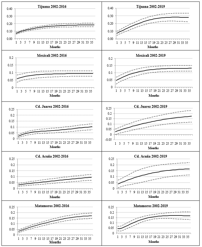
According to INEGI statistics, during 2017 annual prices in border cities rose as follows: Tijuana (8.1%); Matamoros (7.1%); Ciudad Juarez (7.0%); and Ciudad Acuña (7.4%). Those numbers are higher than the country-level average inflation rate that stands at 6.7% during the same period. Figure 2 displays the impulse response functions for the same border cities during the analyzed period. Results indicate that Tijuana has the highest pass-through elasticity value, reaching 0.28% after 36 months. Matamoros and Ciudad Juarez are in second place, with an elasticity of 0.17%, then Ciudad Acuña with a pass-through value of 0.16% and, lastly, Mexicali has an elasticity of 0.13%. It is important to emphasize that pass-through values are statistically significant for most periods in all border cities and their values are above the country average pass-through value. Results in this study are consistent with previous studies, such as Solorzano (2017) who finds statistical significance for border cities, except for Matamoros.
Note: We recognize gasoline prices were liberalized in December 2017, but prices started to increase considerably since January 2017 and sometimes we refer as if the liberalized price period were started since January 2017.
Source: Author´s estimations using data from ENOE, INEGI, IMSS, BLS, World Bank, and Banxico. Black lines are the impulse responses for the inflation rate over 36 months. Gray lines represent a 95 percent confidence interval for the impulse response functions.
Figure 2 Pass-Through Effects in Border Cities: Excluding and Including the Gasoline Price Liberalization Period
If the period after 2017 is eliminated from the sample, important results are obtained. In this scenario, the coefficient for Tijuana becomes 0.18%, Matamoros 0.17%, Ciudad Juarez 0.10%, and Ciudad Acuña and Mexicali 0.09%. These pass-through values are also statistically significant, but their impact on the inflation rate is smaller in comparison with the estimates obtained when the increase of gasoline prices is included in the analysis. There are some hypotheses to consider about why pass-through values are higher when the whole sample is included (2002-2019). In December 2017 gasoline prices were liberalized, but since January 2017 gasoline prices increased surprisingly and not consistent with fluctuations in oil prices. Appendix 1.4 shows the 12-month standard deviation for gasoline prices. Before 2017, the standard deviation values oscillated between 1 and 2, but averaged 4.37 after gasoline prices were liberalized.
5.3 Pass-Through Estimates in Non-Border Cities
Figure 3 shows the effect that a 1% change in the exchange rate has on the inflation rate in 27 non-border metropolitan cities. All the cities included in this study are presented in appendix 1.5, but just the cities with the highest elasticity values are mentioned here. As mentioned previously, results indicate that pass-through values are smaller in non-border cities than those obtained in border cities. The highest elasticity values among all non-border metropolitan cities analyzed are in Morelia (0.14%), Chihuahua (0.13%), Culiacan (0.13%), La Paz (0.12%), Colima (0.11%), Tlaxcala (0.11%), Monterrey, and Querétaro (0.08%) after 36 months, while the pass-through values in the rest of the cities are very small or statistically non-significant.
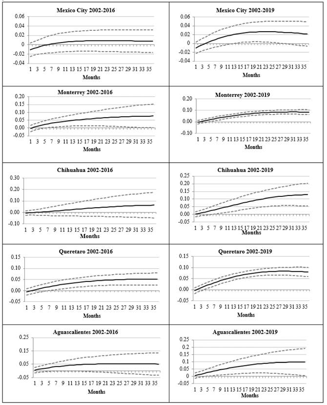
Source: Author´s estimations using data from ENOE, INEGI, IMSS, BLS, World Bank, and Banxico. Black lines are the impulse responses for the inflation rate over 36 months. Gray lines represent a 95 percent confidence interval for the impulse response functions.
Figure 3 Pass-Through Effects in Non-Border Cities: Excluding and Including the Gasoline Price Liberalization Period
When the 2017-19 period is excluded from the analysis, the pass-through estimates for the non-border metropolitan cities become weaker. This is different in comparison with the full sample, where 20 of the 27 cities show a significant relationship. In this case (sub-sample) 7 cities are found to be statistically significant. The impulse response functions are statistically significant only for Colima, Culiacan, Morelia, Monterrey, Queretaro, Torreon, and Merida, where the pass-through values are between 0.03 and 0.08%. Only Culiacan shows a high pass through (0.21%). This value indicates that even if the Mexican peso had depreciated during a portion of the analyzed period, prices would have barely changed in non-border cities. Nevertheless, when gasoline prices increased surprisingly in January 2017 and prices were adjusted to international levels, taxes, etc., producers transferred a portion of the shock, which put pressure on the inflation rate.
It is also important to mention that a different price formation dynamic plays out in Mexico City, Estado de Mexico, Puebla, and Guadalajara in comparison to border cities. There is no clear explanation to clarify such difference in price dynamics. A potential factor could be that in large cities such as Mexico City, Guadalajara, etc. housing is an important factor in the local inflation rate and its connection with the exchange rate is not clearly related.
5.4 Pass-Through values for the entire Border and Non-Border geographic areas
Overall impulse response functions are estimated for the border and non-border cities. In order to obtain those estimates, each city has been weighted according to the National Consumer Price Index (INPC) methodology, the service sector employment share, and large firm employment for each city included in the study. Results indicate that, as expected, pass-through values are higher for border cities than for non-border cities. Elasticity after 36-months is 0.21% for border cities and 0.05% for non-border cities after 18-months. Results are statistically non-significant in the 24th and 36th months in the case of non-border cities.
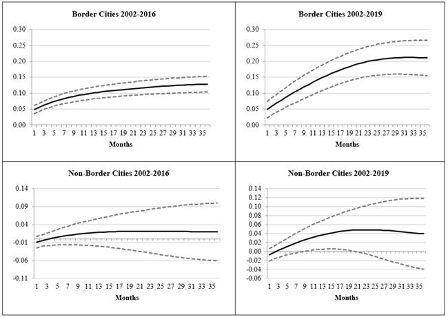
Note: We recognize gasoline prices were liberalized in December 2017, but prices started to increase considerably since January 2017 and sometimes we refer as if the liberalized price period were started since January 2017.
Source: Author´s estimations using data from ENOE, INEGI, IMSS, BLS, World Bank, and Banxico. Black lines are the impulse responses for the inflation rate over 36 months. Gray lines represent a 95 percent confidence interval for the impulse response functions.
Figure 4 Pass-Through Values in Border and Non-Border Cities: Excluding and Including the Gasoline Price Liberalization Period
Figure 4 shows overall estimates for the border and non-border areas during the 2002-2016 and 2002-2019 periods. During the 2002-2016 period (before gasoline shock prices), the exchange rate does not have a statistically significant effect on prices in the case of non-border cities, but when the entire period is included (2002-2019) the effect becomes statistically significant and is close to 0.04%, but does not show significance after the 20th month. In the case of border cities, the effect is statistically significant in both periods, 0-13% for 2002-2016 and above 0.20% for the whole sample (2002-2019) after 36 months.
Distortions in prices after gasoline shock prices (in 2017) plus the lagged exchange rate effects could possibly affect price formation across cities, but higher effects on border cities could be expected. Cortez and Camargo (2009), and Cañas et al. (2013) find that the economic integration between the U.S. and Mexico border cities has increased considerably since 1994 when NAFTA (now called USMCA) came into force. Therefore, border cities could be expected to be more dependent on the U.S. dollar than other Mexican cities.
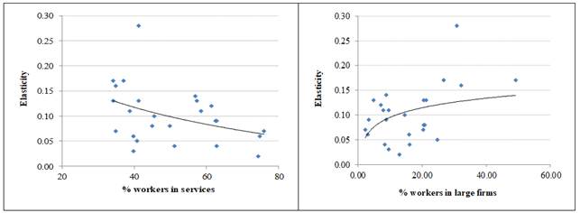
Source: Author´s estimations using data from ENOE, INEGI. We did not consider cities with no significance.
Figure 5 Elasticities and % Workers in Service Sector & Large Firms (2002-2019)
Figure 5 shows a scatter plot for results of the 2002-2019 sample. The y-axis labels for both graphs shows the elasticities for all cities with statistically significant values. The x-axis on the left-hand graph labels the % of workers in the service sector and the right-hand graph labels the % employees of total employees working in large firms. The left-hand graph shows a negative relationship between pass-through values and the percentage of employees in the service sector. The trend line for such scatter plot indicates that an increase in the percentage of employees in the service sector reduces the pass-through elasticities. The right-hand graph shows a positive relationship between the pass-through values and the % employees of total employees in the city working in large firms. The trend line for this graph shows that when more people in a city are working in large firms then the pass-through value increases.
Table 2 Analyzed Period 2002-2019
| % Service Sector Employment in Total Employment | % Large Firms in Total Firms | |
|---|---|---|
| Non-Border Cities | 55% | 15.50% |
| Border Cities | 38% | 27.50% |
Source: Author´s estimations using data from ENOE, INEGI.
Table 2 shows some values which could be helpful to better explain the results found in Figure 5. The second column shows the average proportion of employees among all employees in each border city working in large firms; such average value is 27.50% and is higher by far than the proportion existing in non-border cities which is 15.50%. Large firms are expected to be more dependent on exports/imports (mainly with U.S.) in comparison to small firms. There are some theories that support this argument. For example, Williams (2011) mentions “The statistical analysis revealed that size, not age, has a significant impact on export behavior”. Similarly, Zaclicever (2015) mentions that small and medium firms face several obstacles in international activities in comparison to large firms. Some additional literature that supports the argument that large firms are more involved in international trade in comparison to small and medium firms is Lee et al. (2014) and Ruzzier and Ruzzier (2015). All these results could be helpful to explain the pass-through values obtained in border cities.
Another factor that could be helpful to explain why border cities show a higher pass-through value in comparison to the values obtained for non-border cities is related with the importance of the service sector in the local economy. Results in Table 2 indicate that the service sector in border cities represents, on average, 38% of the total economic activity and 55% in the case of non-border cities. Capistrán (2012) and Cortés (2013) find no relationship between exchange rate and CPI in the service sector CPI or non-tradable goods. Similarly, Solorzano (2017) finds a small or not significant pass-through effect for the service sector and a positive pass-through value in the manufacturing sector.
6. Conclusion
Most of the literature about Mexico regarding pass-through elasticities between the exchange rate and inflation rate has been focused on analyzing the entire country and just a few studies have analyzed the heterogeneity of pass-through values across different geographic regions around Mexico. This study is innovative and different from previous ones because it compares CPIs in cities that are expected to be more dollar dependent (border cities) and cities that are expected to be less dollar dependent (non-border cities). In addition, the analysis includes a period (2017-2019) where gasoline prices increased considerably and then liberalized late in December 2017 and increased by 18% starting in January 2017 and the country inflation rate increased to nearly 7% in that year, a level not seen since 2008. For such reason, the analysis differentiates between the 2002-2016 sample and the 2002-2019 sample period.
Results indicate that the accumulated pass-through elasticity of Mexico's CPI during the 2002-2019 period is 0.07%, a small pass-through value even though it was influenced by the 8% appreciation in the Mexican peso against the U.S. dollar in 2017. Results also indicate that pass-through values are somewhat higher in border cities than in non-border cities. Tijuana, Ciudad Juarez, and Matamoros are the three border cities with the highest impulse response functions during the analyzed period. When the sample is split between the period before and after gasoline increased sharply in January 2017, pass-through values are found to be consistently a little higher in all border cities during the latter period.
It can also be mentioned that border cities are smaller in comparison to other larger cities in the country and, consequently, the CPI in those small border cities is more sensitive to exchange rate shocks than elsewhere in the country. Other factors that could be relevant to justify the higher pass-through values found in border cities in comparison to non-border cities are the economic integration that has continuously increased in the last years between the Mexican north border cities and the U.S. south border cities because of NAFTA. A second factor could be related to the small size of the service sector in border cities in comparison to non-border cities. Literature about this was provided which argues that large service sectors in a city could make local economies more independent from external shocks (exchange rate variations). A third factor could be related to the percentage of people among total employees in a city working in large firms. Literature provided about this argues that, in general, large firms are more dependent on international trade (exchange rate variations) than small and medium firms.
Results also indicate that the pass-through effect is smaller or non-significant in non-border cities, such as Ciudad de Mexico, Guadalajara, Puebla, and Toluca. In addition, there are some non-border industrial cities, such as Monterrey, Chihuahua, Torreon, and Queretaro, which show a weak reaction also to exchange rate variations. Results also indicate that the dynamic of prices in cities such as La Paz, Culiacan, Colima, and Morelia is also affected by variations in the exchange rate even though these cities are not industrial cities. Lastly, given the scarcity of studies analyzing the effects of monetary policy at the regional level in Mexico, the results obtained in this study are expected to be relevant for government officials and practitioners and inspire them to develop more research in this direction.