1. Introduction

Power generation is subject to different sources of uncertainty (e.g., changes in fuel and electricity prices, changes in the cost of CO₂ emissions, and changes in the interest rate). Therefore, uncertainty exerts a direct impact on the risk-return profiles of the generation of different technologies. In this regard, the Portfolio Theory, developed by Markowitz (¹⁹⁵²), has been extensively used to design plans for power generation that reduce risk and increase returns through diversification (see DeLlano-Paz et al. (²⁰¹⁷), for a review). However, existing papers do not provide a description on how the authors construct the Efficient Frontier (EF) of the Power Generation Portfolio (PGP) analyzed (e.g., Perea González and Zavaleta Vazquez (²⁰²⁰), Gómez-Ríos and Juárez-Luna (²⁰¹⁹), Costa et al. (²⁰¹⁷), Pinheiro Neto et al. (²⁰¹⁷), Adams and Jamasb (²⁰¹⁶), Jain et al. (²⁰¹⁴), Cunha and Ferreira (²⁰¹⁴), Francés et al. (²⁰¹³), Losekann et al. (²⁰¹³), Arnesano et al. (²⁰¹²), Bhattacharya and Kojima (²⁰¹²), Allan et al. ( ²⁰¹¹), Delarue et al. (²⁰¹¹), Roques et al. (²⁰¹⁰), Vithayasrichareon et al. (^2010a), Vithayasrichareon et al. (^2010b), Roques et al. (²⁰⁰⁸), Roques (²⁰⁰⁶), and Awerbuch and Berger (²⁰⁰³)). The construction of the EF, performed mostly by simulation, remains as a black box.

In the present paper, we aim to open such a black box by providing a detailed methodology for the parametric construction of the EF of PGP of up to five assets.¹ Following the existing literature, in the present analysis the EF refers to the set of the PGP that maximize their expected returns for a given level of risk. That is, the expected return of an efficient PGP can be increased only by increasing its risk (^{Awerbuch and Berger, 2003}). The present methodology could also be applied to PGP based on the Levelized Cost of Electricity (LCOE). In such a case, the EF would be a set of PGP that can yield the lowest expected LCOE at given levels of expected risk (^{Jansen et al., 2006}).

The analysis relies on the fact that the risk of the PGP is a convex function of the shares of the different assets. The methodology works as follows: first, obtain the shares of the assets that guarantee the maximal expected return on the PGP. Then, obtain the shares of the assets that guarantee the minimal risk of the PGP. We then formulate the risk of the efficient generation portfolios as a parametric equation of the shares of the assets. Finally, the EF corresponds to the parametric equation of the risk-return profiles from the minimal risk of the PGP to the maximal expected return of the PGP.

The majority of the existing literature on energy portfolios follows a two-step methodology proposed by Roques et al. (²⁰⁰⁸). In the first step, the distribution of the returns is simulated by applying Monte Carlo simulation or real options theory. In the second step, the portfolio theory is applied to simulated data to find the optimal generation portfolios. In this paper we focus on the second step of such a methodology.

To exemplify the advantages and the scope of the methodology, we apply it to replicating and extending the existing results from the following three papers: Roques et al. (²⁰⁰⁸), Jain et al. (²⁰¹⁴), and Roques et al. (²⁰¹⁰). Among the main results, we have the following:

Roques et al. (²⁰⁰⁸) analyze portfolios of three technologies: CyCle gas turbine (CCGT), coal, and the nuclear plant. These authors conduct the analysis with pairs of technologies under three scenarios as follows: a) no correlation among the prices of electricity, fuel and CO₂; 2) there are correlations among the prices of electricity, fuel and CO₂, and 3) investors can secure a long-term power purchase agreement. We replicate the results of the second scenario. Our results contradict the following conclusion of Roques et al. (²⁰⁰⁸): "the optimal portfolio for an investor in this case study is to invest only in CCGTs, as any other portfolio would both reduce returns and increase risk." We find efficient portfolios that assign to CCGT a share less than 100%. Actually, the efficient portfolio of minimal risk and also minimal Expected Net Present Value (ENPV) has the following shares: CCGT 53.7%, nuclear 20.5%, and coal 25.8%.

Jain et al. (²⁰¹⁴) analyze portfolios of four types of nuclear reactors: 1) Generic Gen III type Light Water Reactor (LWR); 2) Fast Reactors (FR); 3) High Temperature Reactor (HTR), and 4) Super Critical Water Reactor (SCWR). The analysis was conducted under budget constraint and capacity constraint.² We replicate the results of the case with budget constraint. The EF we obtain differs considerably from the one obtained by Jain et al. (²⁰¹⁴). We find that the portfolio of minimal risk and lower expected return has the following shares: Gen III 18%, HTR 26%, SCWR 25%, and FR 31%. This result contradicts the following conclusion of Jain et al. (²⁰¹⁴): "an investor who wants to minimize the uncertainty of returns and is willing to take a lower expected return in order to do so,will choose a portfolio with more Gen IV type reactors [FR 56% and HTR 35%]."

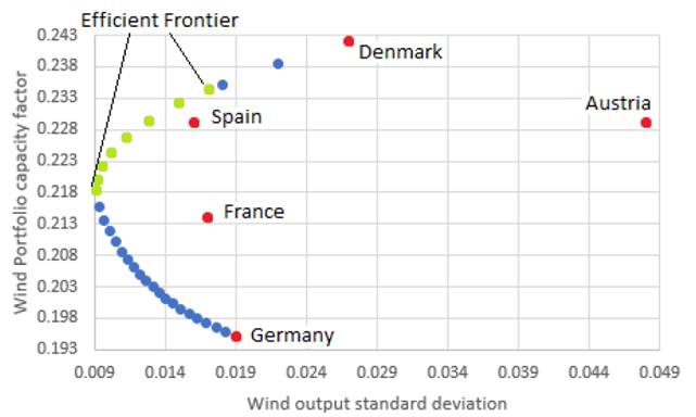
Roques et al. (²⁰¹⁰) analyze cross-country portfolios of joint wind production of five European countries (Austria, Denmark, France, Germany, and Spain). The authors utilize two objective functions to define optimal cross-countries wind power portfolios: i) optimizing wind-power output, and ii) maximizing wind-power contribution to system reliability.³ We replicate the results of the first objective function. Our results are considerably different than the ones obtained by Roques et al. (²⁰¹⁰). For instance, we find that the efficient portfolio that reaches a Wind Portfolio Capacity Factor (WPCF) of 0.2318 allocates the following weights to the five countries: Spain 30%, Germany 8%, Austria 5%, France 7%, and Denmark 50%. On the other hand, Roques et al. (²⁰¹⁰) find that, for the same WPCF level, the efficient portfolio allocates the following weights to the five countries: Spain 54%, Germany 0%, Austria 6%, France 10%, and Denmark 31%. Differences are noteworthy in the weights received by Denmark, Spain, and Germany.

The present methodology has remarkable advantages: 1) it allows to conduct analysis with up to five assets together; 2) it allows to know the shares of the assets for any risk-return profile; 3) the EF is limited by a maximum allowed risk of the PGP; 4) it provides more coherent results than those obtained in the existing literature; 5) it points out that there are optimal investment alternatives that have been denied by previous analysis, and 6) it avoids biases in the design of investment policies in electricity generation. Therefore, the parametric formulation of the EF of the PGP constitutes a powerful tool for both power generation policy-makers and large power companies (in liberalized markets). In addition, the present methodology could be extended to analyze portfolios of more than five asses.

The paper also states that the so-called "portfolio effect" results from the fact that the risk of the PGP is a convex function of the shares of the different assets.

The whole analysis relies on the assumption that the covariances of the returns of the different assets are zero. This strong assumption allows gains in tractability, clarity, and in the scope of the methodology formulated.

To the best of our knowledge, this is the first effort to provide a detailed methodology for the parametric construction of the EF of PGP. It is noteworthy that the present parametric formulation of the EF of PGP could be applied to portfolios based on assets different from those of power-generation technologies.⁴

The paper is organized as follows: in Section 2, we present the preliminaries; Section 3 presents PGP of 2 and 3 technologies, replicates the results obtained by Roques et al. (²⁰⁰⁸), and provides the proof of the "portfolio effect." Section 4 presents PGP of 4 nuclear reactors and replicates the results obtained by Jain et al. (²⁰¹⁴). Section 5 presents cross-country PGP of 5 countries and replicates the results obtained by Roques et al. (²⁰¹⁰). Section 6 contains the final remarks and conclusions. The appendix contains the formal proofs.

2. Preliminaries

We apply the Portfolio Theory developed by Markowitz (¹⁹⁵²) to find the efficient power-generation mix: the return of the generation mix can be increased only by increasing its risk. As customary, risk is measured by the Standard Deviation (SD) of the returns. Formally, let Xi be the random variable that represents the return of asset i and let Y be a random variable describing the return of the PGP, which is defined as follows:

Where αi∈0,1 represents the share of asset i. Following result provides the basic tools for the analysis.

Lemma 1 Let Xi be a random variable that represents the return of asset i with mean μi and variance σi2 . Where αi∈0,1 is the the share of asset i=1,2,…,n . Let the return of the PGP be represented by the random variable Y=∑i=1n‍αiXi with ∑i=1n‍αi=1 . Then

and

where the double summation extends to any values i and j , from 1 to n , such that i<j . In addition, σi,j=EXi-μiXj-μj is the covariance of the returns of assets i and j.

See pp. 158, Freund et al. (²⁰⁰⁰).

The first result of Lemma 1 indicates that the expected return of the PGP is a convex sum of the expected returns of the different assets. Following corollary summarizes such a fact:

Corollary 1 Assume that assets are ordered according to their expected return, μ1≥μ2≥⋯≥μn-1≥μn . Then, it holds that μ1≥μY≥μn.

Second result of Lemma 1 indicates that the risk of the PGP depends on two facts of the different assets, their shares and the covariances of their returns. The risk of the PGP reduces when the covariances among the returns of the assets are negative. The risk of the PGP increases when the covariances among the returns of the assets are positive.⁵ The existing literature reports that, regardless of the variable used to construct the PGP (NPV, LCOE, capacity factor, or installed capacity), the covariances amongst the different assets have an absolute value considerably less than one (e.g., Perea González and Zavaleta Vazquez (²⁰²⁰), Pinheiro Neto et al. (²⁰¹⁷), Adams and Jamasb (²⁰¹⁶), Cunha and Ferreira (²⁰¹⁴), Roques et al. (²⁰¹⁰), and Roques et al. (²⁰⁰⁸)). As the shares of the assets have values less than one, we expect the term ∑‍∑i<j‍αiαjσi,j to be significantly smaller than the term ∑i=1n‍αi2σi2 in the risk of the PGP. This fact is particularly true in two cases: a) when the returns of the PGP are given by the NPVs of the different assets, and b) PGP are based on LCOE of the different assets. Both NPV and LCOE are given in million of dollars or pounds. Therefore, for the present analysis, we assume that the covariances among the different assets is zero, that is, σi,j=0, for any values i and j , from 1 to n, such that i<j. Certainly, this assumption leads to a loss in precision in calculating the minimal risk of the PGP. However, such loss is compensated by gains in tractability, clarity, and in the scope of the methodology formulated.

Lemma 1 and Corollary 1 provide the tools to construct the EF of the PGP parametrically. The methodology works as follows:

1) Rank the assets according to their expected return, μ1≥μ2≥⋯≥μn-1≥μn. Then, the maximal expected return of the PGP is reached when α1=1 and αi=0 for i=2,...,n.

2) Obtain the shares of the assets, αi, that guarantee the minimal risk of the PGP. To do this, we solve the following problem:

3) Formulate the risk of the efficient generation portfolios as a parametric equation of the shares of the assets.

4) Finally, the EF corresponds to the parametric equation of the risk-return profiles from the minimal risk of the PGP to the maximal expected return of the PGP.⁶

Worth noting that, in many cases the EF is not allowed to reach the maximal expected return of the PGP as it is very risky. Under this scenario, we also need to define a maximal allowed risk of the PGP, α1<1, and obtain the corresponding shares of the assets and expected return. In this case the EF corresponds to the parametric equation of the risk-return profiles from the minimal risk of the PGP to the maximal allowed risk of the PGP

Now we have all the building blocks to provide a parametric formulation of the EF of PGP. We start with the portfolios of two technologies.

3. Optimal portfolios for electricity generators in the UK electricity market

In this section we replicate the results obtained by Roques et al. (²⁰⁰⁸). The authors apply portfolio theory to identify the portfolios that maximize the returns of private investors for given risk levels in the UK electricity market. The authors use Monte Carlo simulation to compute the distribution of returns and their correlations. Three technologies are considered: CyCle gas turbine (CCGT), coal, and the nuclear plant. Instead of performing the analysis with the three technologies, these authors work with pairs of plants under three scenarios: 1) no correlation among electricity, fuel and CO₂ prices; 2) there are correlations between electricity, fuel and CO₂ prices, and 3) investors can secure a long-term power purchase agreement.

We replicate the results of the second scenario in which there are correlations among electricity, fuel, and CO₂ prices. Due to expositional motives, we conduct the analysis in two steps. First, as Roques et al. (²⁰⁰⁸) do, we find the efficient portfolios of two technologies: CCGT and coal. Second, we analyze portfolios including those of the three technologies: CCGT, coal and nuclear.

Data is taken from Roques et al. (²⁰⁰⁸), Table 4, 2nd scenario (with correlations), page 1839. The returns and risk of the different generation technologies are given respectively by the ENPV and the SD of the ENPV. The corresponding ENPV and variance of CCGT (cc), Nuclear (nu) and Coal (co) are: μcc=139, μnu=-43, μco=-73, σcc2=2332=54289, σnu2=3772=142129, and σco2=3362=112900.

We proceed to analyze PGP of two technologies.

3.1 Portfolios of two technologies

The risk of the PGP depends on the shares of technologies 1 and 2. The following result provides the shares of technologies 1 and 2 that guarantee the minimal risk of the PGP.

Proposition 1 (Minimal risk of PGP of two technologies) From expression (4) , the risk of a PGP of two technologies is given by σY=∑i=12‍αi2σi2 . Assume that the expected return of technology 1 is the least risky. For σ1,2=0 , αi∈0,1 for i=1,2 , and α1+α2=1 , it holds that

a) The risk of the PGP, given by σY , reaches its global minimum at

α1*α2*=1σ12+σ22σ22σ12

b) The minimal risk of the PGP is

σY*=σ12σ22/σ12+σ22<σ1

See appendix.

The following result provides the parametric formulation of the EF of PGP of two technologies.

Proposition 2 (EF of PGP of two technologies) Let σY=∑i=12‍αi2σi2 be the risk of the PGP. Assume that μ1≥μ2 , thus, the following holds:

a) The risk of the efficient portfolios is obtained by the shares of technologies 1 and 2, given by the following parametric equation:

α1α2=α1-α

where parameter α is such that α1*≤α≤αdf≤1.α1* guarantees the minimal risk of the PGP. While αdf guarantees the maximal allowed risk of the PGP.

b) The risk of the PGP in the EF is given by σYα=α2σ12+1-α2σ22, for α1*≤α≤αdf . Note that σαdf≤σ1.

c) The maximal expected return for each corresponding level of risk is given by μYα=αμ1+1-αμ2, for α1*≤α≤αdf . Note that μαdf≤μ1.

See appendix.

We now have the theoretical tools to analyze the PGP of CCGT and Coal.

3.1.1 Efficient portfolios of CCGT-Coal

Following Proposition 2, CCGT corresponds to technology 1 and Coal to technology 2. Then, from Proposition 1, the shares of the technologies that ensure the minimal risk of the PGP are

αcc*,αco*=0.67528,0.32472

The minimal risk reached by this PGP is σY*=191.47. And the maximal ENPV for such risk is μY=70.159. Note that Roques et al. (²⁰⁰⁸) do not find the minimal risk of the PGP, the shares of the technologies that guarantee such a risk, neither these authors find the corresponding ENPV. They only plot the EF of the PGP.⁷

From Proposition 2, the risk of the efficient portfolios is obtained by the shares of technologies 1 and 2, given by the following parametric equation:

αccαco=α1-α

for 0.67528≤α≤1. Note that the PGP of CCGT-Coal reaches the maximal ENPV when α=αcc=1, and μY=μcc=139. We might say that CCGT "strongly dominates" the PGP, as it has the greatest ENPV, which is also the less risky ENPV. Thus, the risk of the PGP in the efficient frontier is given by 191.47≤σy≤233. The maximal ENPV for each corresponding level of risk is given by 70.159≤μy≤139. The efficient PGP of CCGT-Coal are shown in the following figure:

Figure 1 Efficient PGP of CCGT-Coal 

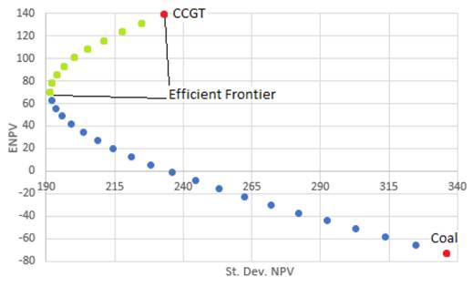
The parameters of the EF are presented in the following figure:

Figure 2 EF of PGP of CCGT-Coal 

Although CCGT strongly dominates the PGP, there are efficient portfolios that assign to CCGT a share less than 100%, which reduce return but also reduce risk. Therefore, CCGT receives a share of 68% in the efficient portfolio of minimal risk and also minimal ENPV. This result contradicts the following conclusion of Roques et al. (²⁰⁰⁸): "The optimal portfolio for an investor in this case study is to invest only in CCGTs, as any other portfolio would both reduce returns and increase risk." In fact, even devoting a share of 100% to CCGT constitutes an efficient portfolio, an economy would face a potential social risk by placing its power generation in one single technology. Thus a decision-maker might support diversification by, for example, allowing the PGP to reach a risk of σy=217.54 and corresponding ENPV μy=123.7. In such a case, the upper limit of the EF would be given by αdf=0.92784 (Figure 2, number 8).

We straightforwardly extend the analysis to the remaining pairs of technologies: CCGT-Nuclear and Nuclear-coal. Following subsection present the EF of every pair of technologies. The corresponding analysis will be provided upon request.

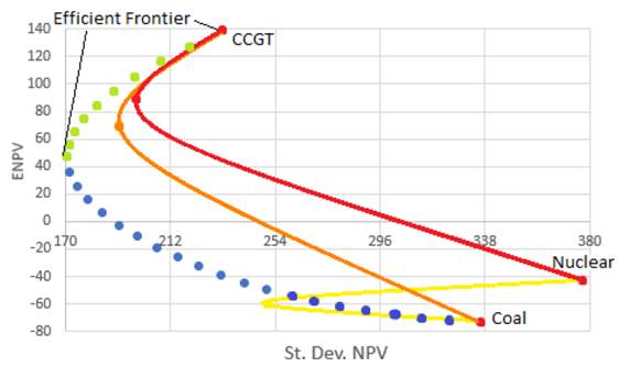
It is noteworthy that the present analysis is incomplete, in that it does not include nuclear plants. The following subsection reveals that introducing nuclear plants changes the shares of the technologies in the efficient portfolios. We now proceed to analyze PGP of three technologies.

3.2 Portfolios of three technologies

The following result provides the shares of technologies 1, 2, and 3, which guarantee the minimum risk of the PGP.

Proposition 3 (Minimal risk of PGP of three technologies) From expression (4) , the risk of the PGP of three technologies is given by σY=∑i=13‍αi2σi2 . Assume that the expected return of technology 1 is the least risky. For σ1,2=σ1,3=σ2,3=0 , αi∈0,1 for i=1,2,3 , and ∑i=13‍αi=1 it holds that

a) The risk of the PGP, given by σY , reaches its global minimum at

α1*α2*α3*=1A3σ22σ32σ12σ32σ12σ22

where A3=σ12σ22+σ12σ32+σ22σ32.

b) The minimal risk of the PGP is

σY*=σ12σ22σ32/A3<σ1

See appendix.

The following result provides the parametric formulation of the EF for PGP of three technologies.

Proposition 4 (EF of PGP of three technologies) Let σY=∑i=13‍αi2σi2 be the risk of the PGP. Assume that μ1≥μ2≥μ3 , thus, the following holds:

a) The risk of the efficient portfolios is obtained by the shares of technologies 1, 2, and 3, given by the following parametric equation:

α1α2α3=α1+xα-α1+x1-α

where parameter α is such that α1*11+x≤α≤αdf≤1 . Let x be given by x=lnα1*/α1*+α2*/lnα1*+α2*.α1*11+x guarantees the minimal risk of the PGP. While αdf guarantees the maximal allowed risk of the PGP.

b) The risk of the PGP in the EF is given by

σYα=α1+x2σ12+α-α1+x2σ22+1-α2σ32,

for α1*11+x≤α≤αdf. Note that σαdf≤σ1.

c) The maximal expected return for each corresponding level of risk is given by μYα=α1+xμ1+α-α1+xμ2+1-αμ3, for α1*11+x≤α≤αdf. Note that μαdf≤μ1.

See appendix.

We now have the tools to analyze the PGP of CCGT-Nuclear-Coal.

3.2.1 Efficient portfolios of CCGT-Nuclear-Coal

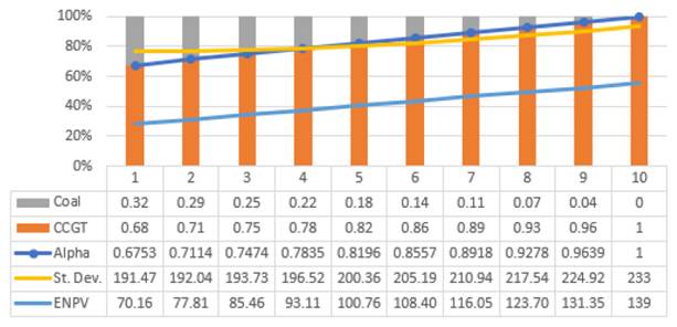
Following Proposition 4, CCGT, nuclear and coal correspond respectively to technologies 1, 2 and 3. Then, from Proposition 3, the shares of the technologies that ensure the minimal risk of the PGP are

αcc*,αnu*,αco*=0.53682,0.20505,0.25813

The minimal risk reached by this PGP is σY*=170.71. The maximal ENPV for such risk is μY=46.957. Roques et al. (²⁰⁰⁸) are not able to find these values because they only carry out the analysis for pairs of technologies.

From Proposition 4, we obtain

x=ln0.53682/0.53682+0.20505/ln0.536 82+0.20505=1.0835

and α1*11+x=0.536 8212. 0835=0.74187. Thus, the risk of the efficient portfolios is obtained by the shares of technologies 1, 2 and 3, given by the following parametric equation:

αccαnuαco=α2.0835α-α2.08351-α

for 0.74187≤α≤1. The PGP of CCGT-Coal-Nuclear reaches the maximal ENPV when α=αcc=1, and μY=μcc=139. Again, we might say that CCGT "strongly dominates" the PGP, as it has the greatest ENPV and the lowest risk. The risk of the PGP in the EF is given by 170.71≤σy≤233. The maximal ENPV for each corresponding risk is given by 46.957≤μy≤139. The efficient PGP of Nuclear-Coal-CCGT are depicted in the following figure:

Figure 3 Efficient PGP of Nuclear-Coal-CCGT 

The triangle in Figure 3 resembles the triangle of the left side of Figure 2, page 841, in Roques et al. (²⁰⁰⁸). However, alike the triangle in Roques et al. (²⁰⁰⁸), we include the PGP of minimal risk for each pair of technologies. The parameters of the EF of the PGP are presented in figure 4.

Figure 4 EF of PGP of Nuclear-Coal-CCGT 

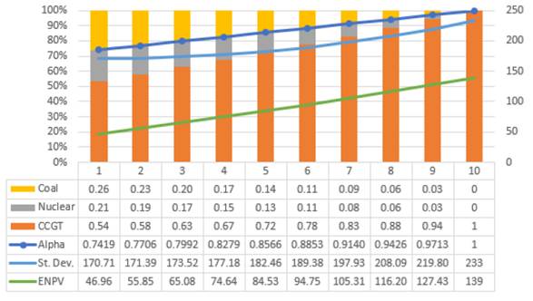
We find that, although CCGT strongly dominates the PGP, there are efficient portfolios that assign to CCGT a share less than 100%, that reduce return but also reduce risk. In fact, the efficient portfolio of minimal risk and also minimal ENPV has the following shares: CCGT 53.7%, nuclear 20.5%, and coal 25.8%. This result contradicts the following conclusion of Roques et al. (²⁰⁰⁸): "The optimal portfolio for an investor in this case study is to invest only in CCGTs, as any other portfolio would both reduce returns and increase risk." Again, a decision-maker might support diversification by, for example, allowing the PGP to reach a risk of σy=208.09 and corresponding ENPV μy=116.2. In such a case, the upper limit of the efficient frontier would be given by αdf=0.94263 (Figure 4, number 8). We find our results more coherent than those obtained by Roques et al. (²⁰⁰⁸).

The present methodology permits the analysis of the PGP of three technologies, providing the shares of the technologies for any risk-return profile in the EF. Thus, there is no need to apply any mean-variance utility function, as Roques et al. (²⁰⁰⁸) do, in order to find efficient portfolios for certain levels of risk aversion. Actually, it would be straightforward to verify that the mean-variance utility function used by Roques et al. (²⁰⁰⁸) reaches its maximum at the efficient portfolio of minimal risk and also minimal ENPV (σY*=170.71 and μY=46.957).

4. Nuclear reactor generation portfolios

In this section we replicate the results obtained by Jain et al. (²⁰¹⁴). The authors apply analyze portfolios of nuclear reactors that maximize the returns for given risk levels. They use real options to compute the distribution of the returns. The following four types of nuclear reactors were considered for the portfolio: 1) Generic Gen III type Light Water Reactor (LWR); 2) Fast Reactors (FR); 3) High Temperature Reactor (HTR), and 4) Super Critical Water Reactor (SCWR). The analysis was conducted under budget constraint and capacity constraint. In this section, we replicate the results of the case with budget constraint.

The risk of the portfolio depends on the shares of reactors 1, 2, 3 and 4. The following result provides the shares of reactors 1, 2, 3 and 4 that guarantee the minimal risk of the PGP.

Proposition 6 (Minimal risk of PGP of four reactors) From expression (4) , the risk of the PGP of four reactors is given by σY=∑i=14‍αi2σi2 . Assume that the expected return of reactor 4 is the least risky. Assume that σi,j=0 , for any values i and j , from 1 to 4, such that i<j . If αi∈0,1 for i=1,2,3,4 , and ∑i=14‍αi=1 it holds that

a) The risk of the PGP, σY , reaches its global minimum at

where A4=σ12σ22σ32+σ12σ22σ42+σ12σ32σ42+σ22σ32σ42.

b) The minimal risk of the PGP is

See appendix.

The following result provides the parametric formulation of the efficient frontier for PGP of four reactors.

Proposition 7 (EF of PGP of four reactors) Let σY=∑i=14‍αi2σi2 be the risk of the portfolio. Assume that μ1≥μ2≥μ3≥μ4 , thus, the following holds:

a) The risk of the efficient portfolios is obtained by the shares of reactors 1, 2, 3 and 4, given by the following parametric equation:

where parameter α is such that α1*11+x1≤α≤αdf≤1 . Let x1 and x2 be given by

α1*11+x1 guarantees the minimal risk of the PGP. While αdf guarantees the maximal allowed risk of the PGP.

b) The risk of the PGP in the EF is given by

for α1*11+x1≤α≤αdf. Note that σαdf≤σ1.

c) The maximal expected return for every corresponding level of risk is given by

for α1*11+x1≤α≤αdf. Note that μαdf≤μ1.

See appendix.

We already have the theoretical tools to replicate the results obtained by Jain et al. (²⁰¹⁴) for the nuclear portfolio of Gen III-HTR-SCWR-FR, under budget constraint. Data is taken from Jain et al. (²⁰¹⁴), Table 11, page 108. The expected returns and variance of reactors Gen III, HTR, SCWR and FR are, respectively: μGenIII=1.3259, μHTR=1.0959, μSCWR=0.972, μFR=0.30778, σGenIII2=1.30362=1.699 4, σHTR2=1.08732=1.182 2, σSCWR2=1.11842=1.2508, and σFR2=0.999252=0.9985.

Following Proposition 7, Gen III, HTR, SCWR, and FR correspond, respectively, to reactors 1, 2, 3, and 4. Thus, from Proposition 6, the shares of the four reactors that ensure the minimal risk are

The minimal risk reached by this PGP is σY*=0.55596. The maximal expected return for such a risk is μY=0.86314. These values are notably different from those obtained by Jain et al. (²⁰¹⁴). These authors find that the minimal risk of the portfolio is 0.95 while the corresponding expected return to such a level of risk is 0.6. These authors also indicate, in Figure 7, that the portfolio of minimal risk and also the minimal return has the following (estimated)⁹ shares: αGenIII,αHTR,αSCWR,αFR=0,0.08,0.37,0.55.

Following Proposition 7, we obtain

and α1*11+x1=0.1818811+1.0953=0.44333. Thus, the risk of the efficient portfolios is obtained by the shares of reactors 1, 2, 3 and 4, given by the following parametric equation:

for 0.44333≤α≤0.8739065. The PGP of Gen III-HTR-SCWR-FR reaches the maximal expected return when α=αGenIII=1, and μY=μGenIII=1.3259. However, to support diversification, the PGP might be allowed to reach a risk of σFR=0.99925, which is the minimal risk of the four nuclear reactor. In this case, the corresponding expected return is μy=11.243144281 and the upper limit of the efficient frontier would be given by αdf=0.8739065. Thus, the risk of the PGP in the EF is given by 0.55596≤σy≤0.99925. The maximal expected return for every corresponding risk is given by 0.86314≤μy≤1.243144281. The efficient PGPs of Gen III-HTR-SCWR-FR are presented in Figure 5.

Figure 5 Efficient PGP of Gen III-HTR-SCWR-FR 

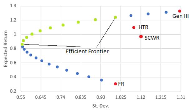
The following figure presents the parameters of the EF. The proposed EF ranges from 1 to 10. Notwithstanding this, we present all of the efficient portfolios in order to compare them with those obtained by Jain et al. (²⁰¹⁴), shown in figure 7b (page 108).

Figure 6 EF of PGP of Gen III-HTR-SCWR-FR 

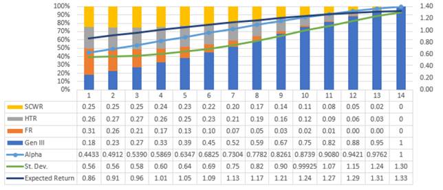
We find that an investor who wants to minimize risk with a lower expected return will chose a portfolio with following shares: Gen III 18%, HTR 26%, SCWR 25%, and FR 31%. This result contradicts the following conclusion of Jain et al. (²⁰¹⁴): "An investor who wants to minimize the uncertainty of returns and is willing to take a lower expected return in order to do so,will choose a portfolio with more Gen IV type reactors [FR 56% and HTR 35%]." Our EF differs considerably from that obtained by Jain et al. (²⁰¹⁴). For example, Jain et al. (²⁰¹⁴) state, in figure 7, that the efficient portfolio that reaches an expected return of 1.2, allocates to reactors Gen III and HTR a share of around 50%. The present analysis indicates that, for such an expected return, the shares of the four reactors are: Gen III 67%, HTR 16%, SCWR 14%, and FR 3%. We find our results more coherent than those obtained by Jain et al. (²⁰¹⁴).

When replicating the case under capacity constraint, we also find different results from those of Jain et al. (²⁰¹⁴). For example, Jain et al. (²⁰¹⁴) state, in figure 8, that the efficient portfolio of minimum risk (σY*=2800) and also minimum expected return (μY=2800) has the following (estimated) shares: Gen III 43%, HTR 8%, SCWR 42%, and FR 7%. On the other hand, we find that the efficient portfolio of minimal risk (σY*=1584.42) and also minimum expected return (μY=2601.18) has the following shares: Gen III 27%, HTR 21%, SCWR 28%, and FR 24% (This case will be provided upon request).

It is noteworthy that the difference in the results creates a bias in the design of investment policies in electricity generation by nuclear reactors.

Jain et al. (²⁰¹⁴) also test the sensitivity of the portfolio under three different scenarios: 1) varying discount rates; 2) varying electricity price growth rates, and 3) varying uncertainties in electricity prices. However, they do not provide the statistics of the returns for such scenarios. The present methodology could be applied to replicate the results of such scenarios if the statistics of the returns were available.

5. Optimal portfolios of wind-power in Europe

In this section, we replicate the results obtained by Roques et al. (²⁰¹⁰). These authors use historical wind-production data from five European countries (Austria, Denmark, France, Germany, and Spain) to identify cross-country portfolios that minimize the risk of joint wind production for a given level of production. They employ two objective functions to define optimal cross-country wind power portfolios: i) optimizing wind-power output, and ii) maximizing wind-power contribution to system reliability. In this section, we replicate the results of the first case.

The risk of the portfolio depends on the weight received by the wind production of countries 1, 2, 3, 4, and 5. The following result provides the weights received by countries 1, 2, 3, 4, and 5 that guarantee the minimal risk of the PGP.

Proposition 8 (Minimal risk of PGP of five countries) From expression (4) , the risk of the PGP of five countries is given by σY=∑i=15‍αi2σi2 . Assume that the expected return of country 3 is the least risky. Assume that σi,j=0 , for any values i and j , from 1 to 5, such that i<j . If αi∈0,1 for i=1,2,3,4,5 , and ∑i=15‍αi=1 it holds that

a) The risk of the PGP, σY , reaches its global minimum at

where A5=σ12σ22σ32σ42+σ12σ22σ32σ52+σ12σ22σ42σ52+σ12σ32σ42σ52+σ22σ32σ42σ52

b) The minimal risk of the PGP is

See appendix.

Following result provides the parametric formulation of the EF of PGP of cross-country wind power.

Proposition 9 (EF of PGP of five countries) Let σY=∑i=15‍αi2σi2 be the risk of the PGP. Assume that μ1≥μ2≥μ3≥μ4≥μ5 , thus, the following holds:

a) The risk of the efficient portfolios is obtained by the weight received by the wind production of countries 1, 2, 3, 4 and 5, given by the following parametric equation:

where the parameter α is such that α1*11+x1+x2≤α≤αdf≤1.

Let x1 , x2 , and x3 be given by

α1*11+x1+x2 guarantees the minimal risk of the PGP, while αdf guarantees the maximal allowed risk of the PGP.

b) The risk of the PGP in the EF is given by

for α1*11+x1+x2≤α≤αdf. Note that σαdf≤σ1.

c) The maximal expected return for every corresponding level of risk is given by

for α1*11+x1+x2≤α≤αdf. Note that μαdf≤μ1.

See appendix.

We now possessed the theoretical tools to replicate the results obtained by Roques et al. (²⁰¹⁰) for the wind portfolios of Denmark-Austria-Spain-France-Germany under the case optimizing wind power output. Data is taken from Roques et al. (²⁰¹⁰), Table 5, page 3250. For these the returns and the risk of the different countries are given by the wind-power capacity factors (WPCF) and their SD. The corresponding expected returns and variance of Denmark, Austria, Spain, France, and Germany are: μDn=0.242, μAu=0.229, μSp=0.229, μFr=0.214, μGr=0.195, σDn2=0.0272=7. 29×10-4, σAu2=0.0482=2. 304×10-3, σSp2=0.0162=2. 56×10-4, σFr2=0.0172=2. 89×10-4, and σGr2=0.0192=3. 61×10-4.

From Proposition 9, countries 1, 2, 3, 4, and 5 correspond, respectively, to Denmark, Austria, Spain, France, and Germany. Thus, from Proposition 8, the weights received by the wind production of the countries that ensure the minimal risk are

The minimal risk of this PGP is given by σY*=0.0091507. And the maximal expected WPCF for such level of risk is μY=0.21826. These values are different from those obtained by Roques et al. (²⁰¹⁰). These authors find that the minimal risk of the portfolio is somewhat greater that 0.01 while the corresponding expected return to such a level of risk is 0.2190. They also indicate, in Figure 4, that the portfolio of minimal risk and also the minimal return has the following (estimated) weights: αDn,αAu,αSp,αFr,αGr=0.09,0.03,0.39,0.29,0.2.

From Proposition 9, we obtain

and α1*11+x1+x2=0.114 8611+1.0417+6.1585=0.76805. Thus, the risk of the efficient portfolios is obtained by the weights received by the wind production of countries 1,2,3,4 and 5, given by the following parametric equation:

for 0.76805≤α≤0.94105. The PGP of Denmark-Austria-Spain-France-Germany reaches the maximal WPCF when α=αDn=1, and μY=μDn=0.242. However, to support diversification, the PGP might be allowed to reach a risk of σFR=0.17, that is, one of the less risky countries. In this case, the corresponding WPCF is μy=0.2343 and the upper limit of the EF would be given by αdf=0.94105. Thus, the risk of the PGP in the EF is given by 0.0091507≤σy≤0.17. The maximal expected return for each corresponding risk is given by 0.218 26≤μy≤0.2343. The following figure presents the efficient PGP of cross-country wind-power.

Figure 7 Efficient PGP, Dn-Au-Sp-Fr-Gr 

The following figure presents the parameters of the EF. The proposed EF ranges from 1 to 8. However, we present all of the efficient portfolios in order to compare them with those obtained by Roques et al. (²⁰¹⁰), shown in figure 4 (page 3251).

Figure 8 EF of PGP, Dn-Au-Sp-Fr-Gr 

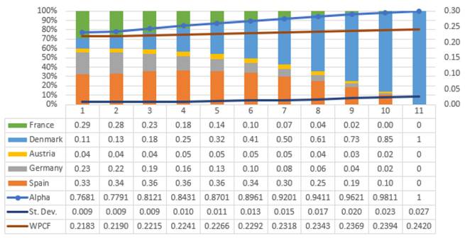
We obtain a very different EF from that obtained by Roques et al. (²⁰¹⁰). For example, we find that the efficient portfolio that reach a WPCF of 0.2318 allocates the following weights to the five countries: Spain 30%, Germany 8%, Austria 5%, France 7%, and Denmark 50%.On the other hand, Roques et al. (²⁰¹⁰) find that, for the same level of WPCF, the efficient portfolio allocates the following weights to the five countries: Spain 54%, Germany 0%, Austria 6%, France 10%, and Denmark 31%. The differences are noteworthy in the weights received by Denmark, Spain, and Germany. In our analysis, Germany receives a weight greater than zero while the weights received by Denmark and Spain are nearly switched between each other in the paper by Roques et al. (²⁰¹⁰).

We find our results more coherent than those obtained by Roques et al. (²⁰¹⁰). To see this, recall the fact that the expected return of the PGP is a convex sum of the expected returns of the different assets. Thus, as the WPCF of 0.2318 is closer to the expected return of Denmark and above the expected return of Spain, we expect that Denmark should receive a greater weight than Spain in the PGP. Which hold in our analysis as the grater weight received by Spain is 33%.

When replicating the case of maximizing the wind-power contribution to the reliability of the system, we also find different results from those of Roques et al. (²⁰¹⁰). Unlike these authors, we find that Germany receives a weight greater than zero and up to 15% in the PGP (This case will be provided upon request).

Notably, the difference in the results creates a bias in the design of policies in electricity generation by cross-country wind-power.

Roques et al. (²⁰¹⁰) also find the EF of "constrained" portfolios. These authors consider two types of constraints: 1)wind resource potential constraints, and 2) network limitations constraints. However, they do not provide the statistics of the returns for each scenario. The present methodology could be applied to replicate the results of such scenarios if the statistics of the returns were available.

6. Final remarks and conclusions

The present paper tackles the problem of the diversification of energy generation by providing a methodology to construct parametrically the EF of PGP for up to five assets. The methodology was applied to replicate and extend the results of the following three papers: Roques et al. (²⁰⁰⁸), Jain et al. (²⁰¹⁴), and Roques et al. (²⁰¹⁰). The present methodology has remarkable advantages:

Thus, the parametric formulation of PGP proved to be a powerful tool for power generation policy-makers or investors. In fact, it could be applied to portfolios of assets different than those of power-generation technologies.

From the structure of the paper, it would be straight forward to extend the methodology to obtaining the shares of assets in order to guarantee the minimal risk of PGP of more than five assets. However, the corresponding mathematical proofs must be performed to construct the EF of PGP parametrically of more than five assets.

Complete analysis relies on the assumption that the covariances of the returns amongst the different assets is zero. Depending on computational availability, future research could be extended to verify the actual effect of the correlations of the returns on the minimal risk of the portfolio.

References

Adams, R., Jamasb, T. 2016. Optimal Power Generation Portfolios with Renewables: An Application to the UK, Cambridge Working Papers in Economics 1646, Faculty of Economics, University of Cambridge. http://www.econ.cam.ac.uk/research-files/repec/cam/pdf/cwpe1646.pdfLinks ]
Allan, G., Eromenko, I., McGregor, P., Swales, K., 2011. The regional electricity generation mix in Scotland: A portfolio selection approach incorporating marine technologies. Energy Policy 39: 6-22. https://doi.org/10.1016/j.enpol.2010.08.028. [ Links ]
Arnesano, M., Carlucci A. P., Laforgia D., 2012. Extension of portfolio theory application to energy planning problem - The Italian case. Energy 39: 112-114. doi: https://doi.org/10.1016/j.energy.2011.06.053Links ]
Awerbuch, S., Berger, M., 2003. Applying portfolio Theory to EU Electricity Planning and Policy-Making. IEA/EET Working Paper. IEA. Paris. https://pdfs.semanticscholar.org/0ca8/8df704e4f08ebb458bcf8c4cc418f3eaa634.pdf?_ga=2.112372356.1645367726.1590520337-1249187651.1590520337Links ]
Bhattacharya A., Kojima S., 2012. Power sector investment risk and renewable energy: A Japanese case study using portfolio risk optimization method. Energy Policy 40: 69-80. doi:https://doi.org/10.1016/j.enpol.2010.09.031Links ]
Costa, O. L.V., Ribeiro, C. O., Rego, E. E., Stern, J. M., Parente, V., Kileber, S., 2017. Robust portfolio optimization for electricity planning: An application based on the Brazilian electricity mix. Energy Economics 64: 158-169. doi:https://doi.org/10.1016/j.eneco.2017.03.021Links ]
Cunha, J., Ferreira, P., 2014. Designing electricity generation portfolios using the mean-variance approach, Int. J. Sustain. Energy Plan. Manag., 4: 17-30. doi:https://doi.org/10.5278/ijsepm.2014.4.3Links ]
Delarue E., Jonghe C., Belmans R., D’haeseleer W., 2011. Applying portfolio theory to the electricity sector: Energy versus power. Energy Economics 33: 12-23. doi:https://doi.org/10.1016/j.eneco.2010.05.003Links ]
DeLlano-Paz, F., Calvo-Silvosa, A., Antelo, S. I., Soares, I., 2017. Energy planning and modern portfolio theory: A review. Renewable and Sustainable Energy Review 77: 636-651. doi:https://doi.org/10.1016/j.rser.2017.04.045Links ]
Francés G. E., Marín-Quemada J.M., González E. S., 2013. RES and risk: Renewable energy’s contribution to energy security. A portfolio based approach, Renewable and Sustainable Energy Reviews 26: 549-559. doi:https://doi.org/10.1016/j.rser.2013.06.015Links ]
Freund, J. E., Miller, I, Miller, M., 2000. Estadística matemática con aplicaciones. Pearson educación. [ Links ]
Gómez-Ríos, M., and Juárez-Luna, D. (2019). Cost of electric generation accounting for environmental externalities: Optimal mix of baseload technologies. Revista Mexicana de Economía y Finanzas Nueva Época REMEF, 14(3), 353-377. doi:https://doi.org/10.21919/remef.v14i3.308Links ]
Jain, S., Roelofs, F., Oosterlee, C. W., 2014. Decision-support tool for assessing future nuclear reactor generation portfolios. Energy Economics 44: 99-112. doi:https://doi.org/10.1016/j.eneco.2014.03.021Links ]
Jansen, J. C., Beurskens, L.W.M., Tilburg, X.V., 2006. Application of portfolio analysis to the Dutch generating mix. ECN report C-05-100. Energy research council of Netherlands. https://publicaties.ecn.nl/PdfFetch.aspx?nr=ECN-C-05-100Links ]
Losekann L., Marrero G. A., Ramos-Real F. J., Almeida E. L., 2013. Efficient power generating portfolio in Brazil: Conciliating cost, emissions and risk. Energy Policy 62: 301-314. doi:https://doi.org/10.1016/j.enpol.2013.07.049Links ]
Markowitz H. M., 1952. Portfolio Selection, Journal of Finance, Vol. 7, pp 77-91. DOI: 10.2307/2975974Links ]
Perea González, A., and Zavaleta Vazquez, O. (2020). Designing an optimal electricity supply portfolio based on the Markowitz model: The case of a user in Mexico. Contaduría y Administración, 65(1), 1-20. doi:http://dx.doi.org/10.22201/fca.24488410e.2019.1833Links ]
Pinheiro Neto, D., Domingues, E. G., Coimbra, A. P., de Almeida, A. T., Alves, A. J., Calixto, W. P., 2017. Portfolio optimization of renewable energy assets: hydro, wind, and photovoltaic energy in the regulated market in Brazil. Energy Economics 64: 238-250. doi:https://doi.org/10.1016/j.eneco.2017.03.020Links ]
Roques, F. A., Hiroux, C., Saguan, M., 2010. Optimal wind power deployment in Europe - A portfolio approach, Energy Policy 38: 3245-3256. doi:https://doi.org/10.1016/j.enpol.2009.07.048Links ]
Roques, F. A., Newbery, D. M., Nuttall, W. J., 2008. Fuel mix diversification incentives in liberalized electricity markets: A Mean-Variance Portfolio theory approach, Energy Economics, Volume 30, Issue 4: 1831-1849. doi:https://doi.org/10.1016/j.eneco.2007.11.008Links ]
Roques, F. (2006). Power generation investments in liberalised markets: methodologies to capture risk, flexibility, and portfolio diversity. Économies et Sociétés, Série Economie de l’Energie 10 (Oct./Nov.), 1563-94. [ Links ]
Vithayasrichareon, P., MacGill, I.F., Wen, F.S., 2010a. Electricity generation portfolio evaluation for highly uncertain and carbon constrained future electricity industries. IEEE Power and Energy Society General Meeting. doi:https://doi.org/10.1109/pes.2010.5589354Links ]
Vithayasrichareon, P., MacGill, I.F., Wen, F., 2010b. Electricity Generation Portfolio Analysis for Coal, Gas and Nuclear Plant under Future Uncertainties. 4th IASTED Asian Conference on Power and Energy Systems. doi:https://doi.org/10.2316/p.2010.701-027Links ]
1Depending on the context, the assets could be technoologies, reactors, or wind production of countries.
2See Jain et al. (2014) for the details of the different reactors and the different constraints.
3See Roques et al. (2010) for the details of the different objective functions.
4For instance, it could be employed to analize portfolios of five electricity suppliers as those studied by Perea González and Zavaleta Vazquez (2020).
5Roques (2006) shows efficient frontier of PGP of CCGT- nuclear for various degrees of hypotetical returns correlation.
6When the PGP is based on LCOE, the ranking of the expected LCOE is as follows: μ1μ2μn-1μn. In this case, the EF corresponds to the parametric equation of the risk-cost profiles from the minimal risk of the PGP to the minimal expected LCOE of the PGP.
7See Figure 2, page 841, in Roques et al. (2008).
8In this regard, Gómez-Ríos and Juárez-Luna (2019) also analyze pairs of three available technologies. Then, their results are also incomplete.
9We mention that the shares are "estimated", in that, of not having the true values, we obtained them from the graph.
Appendix
[Proof of Proposition 1] The risk of the PGP of two technologies is given by σY=α12σ12+α22σ22. Assume that the expected return of technology 1 is the least risky. For σ1,2=0, αi0,1 for i=1,2, and α1+α2=1. For tractability, the majority of the proof uses the variance of the PGP instead of its SD.
Proof of a) We need to find the shares of technologies 1 and 2, given by α1,α2, which guarantee the minimum risk (variance) of the PGP. For tractability, take α2=1-α1. Then, the risk of the PGP is given by σY2=α12σ12+1-α12σ22. First, we find the critical point of the risk of the PGP. The First Order Conditions (FOC) are as follows:
σY2/α1=2α1σ12+21-α1-1σ22=0 (5)
From expression (5), we have
α1σ12+α1σ22=σ22 (6)
which leads to
α1*=σ22/σ12+σ22 (7)
Thus, α2*=1-α1*=σ12/σ12+σ22. The critical point of the risk of the PGP is given by shares
α1*,α2*=1/σ12+σ22σ22,σ12 (8)
To verify that the risk of the PGP, σY2 has a minimum at the critical point α1*,α2*, we need the Second Order Conditions (SOC):
2σY2/α12=2σ12+σ22>0
Thus, the risk of the PGP is a convex function of the shares of the two technologies, α1,α2. As a consequence, the risk of the PGP, σY2 has a global minimum when the shares of technologies 1 and 2 are given by expression (8).
Proof of b) Thus, the minimal risk of the PGP, σY*2, is given by
σY*2=1/σ12+σ222σ222σ12+σ122σ22,
σY*2=σ12σ22/σ12+σ222σ22+σ12,
σY*2=σ12σ22/σ12+σ22=α1*σ12<σ12,
Then
σY*<σ1. (9)
The minimal risk of the PGP is lower than the risk of the least risky technology.
[Proof of Proposition 2] Let σY=α12σ12+α22σ22 be the risk of the PGP of two technologies. From Proposition 3, we know that the risk of the PGP, σY, reaches its global minimum at point α1*,α2*. Assume that μ1μ2.To obtain the parametric formulation of the EF, we express the risk of the PGP as follows:
σY2=α2σ12+1-α2σ22, (10)
for α0,1. Note that when α=1, then σY2=σ12, the risk of the PGP equals the risk of technology 1. This scenario ensures that technology 1, which has the greatest expected return, receives a share of 100%. On the other hand, when α=0, then σY2=σ22, the risk of the PGP equals the risk of technology 2. The latter implies that technology 2, which has the lowest expected return, receives a share of 100%. Thus, this formulation of the risk of the PGP allows to have portfolios assigning a share of 100% to the technologies with the greatest and least expected return. We need to ensure that expression (10) allows to reach the point α1*,α2* where σY reaches its global minimum. Then, it should hold that
α1*=α, (11)
α2*=1-α, (12)
Expressions (11) and (12) lead to the fact that the shares of technologies 1 and 2 in the risk of the PGPs are given by
α1=α, (13)
α2=1-α, (14)
Then, from expression (10) the risk of the PGP is given by
σY2=α2σ12+1-α2σ22, (15)
From expressions (11) and (13), the PGP with lowest risk is given by
α=α1*. (16)
Now we need to find the PGP with the greatest expected return. The expected return of the PGP is given by:
μY=α1μ1+α2μ2, (17)
substituting expressions (13) and (14) in expression (17) leads to
μY=αμ1+1-αμ2, (18)
it is straightforward to obtain that
dμY/dα=μ1-μ20,
because of the assumption that μ1μ2. Then, the PGP reaches its maximum expected return when α=1, μY=μ1, and σY2=σ12. However, there could be an alternative criterion to choose the maximal expected return of the PGP. For example, if the expected return of technology 1 is the least risky, then, the criterion could be to choose αdf, so that σY2αdf=σ12; in this case, αdf<1. Then, the corresponding maximal expected return of the PGP is given by μαdf. Thus, the risk of the efficient portfolios is obtained by the shares of technologies 1 and 2, given by expressions (13) and (14) for α1*ααdf. As a consequence, the risk of the PGP in the EF is given by expression (15). The maximal expected return for each corresponding level of risk is given by expression (18). Note that μαdfμ1 and σαdfσ1.
[Proof of Proposition 3] The risk of the PGP of three technologies is given by σY=i=13αi2σi2. Assume that the expected return of technology 1 is the least risky. For σ1,2=σ1,3=σ2,3=0, αi0,1 for i=1,2,3, and i=13αi=1. For tractability, the majority of the proof uses the variance of the PGP instead of its SD.
Proof of a) We need to find the shares of technologies 1, 2, and 3, given by α1,α2,α3, which ensures the minimum risk (variance) of the PGP. For tractability, take α3=1-α1-α2. Then, the risk of the PGP is given by σY2=α12σ12+α22σ22+1-α1-α22σ32. First, we find the critical point of the risk of the PGP. The FOC are the following:
σY2/α1=2α1σ12+21-α1-α2-1σ32=0, (19)
σY2/α2=2α2σ22+21-α1-α2-1σ32=0, (20)
from expression (19), we have
α1σ12+σ32+α2σ32=σ32, (21)
from expression (20), we have
α1σ32+α2σ22+σ32=σ32. (22)
Expressions (21) and (22) lead to the following system of equations
σ12+σ32σ32σ32σ22+σ32α1α2=σ32σ32, (23)
Calculating the inverse of matrix A3=σ12+σ32σ32σ32σ22+σ32 we end up with
α1*α2*=1A3σ22+σ32-σ32-σ32σ12+σ32σ32σ32, (24)
where A3=σ12σ22+σ12σ32+σ22σ32, leading to the result
α1*α2*=1A3σ22σ32σ12σ32. (25)
Then, α3*=1-α1*-α2*=σ12σ22/A3. The critical point of the risk of the PGP is given by shares
α1*,α2*,α3*=1/A3σ22σ32,σ12σ32,σ12σ22. (26)
To verify that the risk of the PGP, σY2, has a minimum at the critical point α1*,α2*,α3*, we need the SOC. The Hessian matrix is given as follows:
H=2σ12+σ32σ32σ32σ22+σ32,
Following the criteria of the leading principal minors of the Hessian matrix, we have
H1=2σ12+σ32>0.
H2=2A3=2σ12σ22+σ12σ32+σ22σ32>0.
The two leading principal minors of the Hessian matrix are positive for any α1,α2,α3. Thus, the risk of the PGP is a convex function of the shares of the three technologies, α1,α2,α3. As a consequence, the risk of the PGP, σY2, has a global minimum when the shares of technologies 1, 2, and 3 are given by expression (26).
σY*2=1/A32σ22σ322σ12+σ12σ322σ22+σ12σ222σ32,
σY*2=σ12σ22σ32/A32σ12σ22+σ12σ32+σ22σ32,
σY*2=σ12σ22σ32/A3=α1*σ12<σ12,
σY*<σ1. (27)
[Proof of Proposition 4] Let σY=i=13αi2σi2 be the risk of the PGP of three technologies. From Proposition 5, we know that the risk of the PGP, σY, reaches its global minimum at point α1*,α2*,α3*. Assume that μ1μ2μ3 . To obtain the parametric formulation of the EF, we express the risk of the PGP as follows:
σY2=α2β2σ12+1-β2σ22+1-α2σ32,σY2=α2β2σ12+α21-β2σ22+1-α2σ32, (28)
for α,β0,1. Note that when α=β=1, then σY2=σ12, the risk of the PGP equals the risk of technology 1. This scenario implies that technology 1, which has the greatest expected return, receives a share of 100%. On the other hand, when α=0, then σY2=σ32, the risk of the PGP equals the risk of technology 3. Then, technology 3, which has the lowest expected return, receives a share of 100%. Thus, this formulation of the risk of the PGP allows to have portfolios that assign a share of 100% to the technologies with the greatest and least expected return. We need to ensure that expression (28) allows to reach the point α1*,α2*,α3*, where σY reaches its global minimum. Then, it should hold that
α1*=αβ, (29)
α2*=α1-β, (30)
α3*=1-α, (31)
from expression (29)
α=α1*/β (32)
substituting expression (32) in expression (30) leads to
β=α1*/α1*+α2*, (33)
substituting expression (33) in expression (32) leads to
α=α1*+α2*. (34)
To ensure that β0,1 for α0,1, assume that
β=βα=αx (35)
Then, substituting expressions (33) and (34) in expression (35) we have
α1*/α1*+α2*=α1*+α2*x.
x=lnα1*/α1*+α2*/lnα1*+α2*. (36)
Substituting expression (35) in expressions (29), (30), and (31) leads to the fact that the shares of technologies 1, 2 and 3 in the risk of the PGP are given by the following expressions:
α1=αβ=α1+x, (37)
α2=α1-β=α-α1+x, (38)
α3=1-α. (39)
Then, substituting expressions (37), (38), and (39) into (28) leads to the risk of the PGP:
σY2=α1+x2σ12+α-α1+x2σ22+1-α2σ32. (40)
From expressions (29) and (37), the PGP with lowest risk is given when
α=α1*11+x. (41)
μY=α1μ1+α2μ2+α3μ3, (42)
substituting expressions (37), (38), and (39) in expression (42) leads to
μY=α1+xμ1+α-α1+xμ2+1-αμ3, (43)
It is straightforward to obtain that
dμY/dα=1+xαxμ1-μ2+μ2-μ30,
because of the assumption that μ1μ2μ3. Then, the PGP reaches its maximum expected return when α=1, μY=μ1 and σY2=σ12. However, there could be an alternative criterion to choose the maximal expected return of the PGP. For example, if the expected return of technology 1 is the least risky, then, the criterion could be to choose αdf, so that σY2αdf=σ12, in this case αdf<1. Then, the corresponding maximal expected return of the PGP is given by μαdf. Thus, the risk of the efficient portfolios is obtained by the shares of technologies 1, 2, and 3, given by expressions (37), (38), and (39) for α1*11+xααdf. As a consequence, the risk of the PGP in the EF is given by expression (40). The maximal expected rerun for each corresponding level of risk is given by expression (43). Note that μαdfμ1 and σαdfσ1.
[Proof of Proposition 5] We conducted the proof for PGP of three technologies. However, it is straightforward to extend the proof to PGP of more than three technologies. Consider three-power generation technologies with corresponding risks σ12, σ22, and σ32. The minimal risk reached by a PGP consisting of technology 1 is σY1*=σ1. From proposition 3b, the minimal risk reached by a PGP of two technologies is σY2*=σ12σ22/σ12+σ22. From proposition 5b, the minimal risk reached by a PGP of three technologies is σY3*=σ12σ22σ32/A3, where A3=σ12σ22+σ12σ32+σ22σ32. We need to prove that σY1*>σY2*>σY3*.
a) First, we verify whether σY1*>σY2* holds:
σ1>σ12σ22/σ12+σ22,σ12>σ12σ22/σ12+σ22,σ14+σ12σ22>σ12σ22,σ14>0.
Then, it holds that σY1*>σY2*.
b) Second, we verify whether σY2*>σY3* holds:
σ12σ22/σ12+σ22>σ12σ22σ32/A3,σ12σ22/σ12+σ22>σ12σ22σ32/A3,σ14σ24+σ14σ22σ32+σ12σ24σ32>σ14σ22σ32+σ12σ24σ32,σ14σ24>0.
Then, it holds that σY2*>σY3*. It follows that σYn*<σYk* for k<n.
[Proof of Proposition 6] The risk of the PGP of four nuclear reactors is given by σY=i=14αi2σi2. Assume that the expected return of reactor 4 is the least risky. If σi,j=0, for any values i and j, from 1 to 4, such that i<j. If αi0,1 for i=1,2,3,4, and i=14αi=1. For tractability, the majority of the proof uses the variance of the PGP instead of its SD.
Proof of a) We need to find the shares of reactors 1, 2, 3 and 4, given by α1,α2,α3,α4, which ensures the minimum risk (variance) of PGP. For tractability, take α4=1-α1-α2-α3. Then, the risk of the PGP is given by σY2=α12σ12+α22σ22+α32σ32+1-α1-α2-α32σ42. First, we find the critical point of the PGP. The FOC are the following:
σY2/α1=2α1σ12+21-α1-α2-α3-1σ42=0, (44)
σY2/α2=2α2σ22+21-α1-α2-α3-1σ42=0, (45)
σY2/α3=2α3σ32+21-α1-α2-α3-1σ42=0, (46)
from expression (44), we have
α1σ12+σ42+α2σ42+α3σ42=σ42, (47)
from expression (45), we have
α1σ42+α2σ22+σ42+α3σ42=σ42, (48)
from expression (46), we have
α1σ42+α2σ42+α3σ32+σ42=σ42. (49)
Expressions (47), (48), and (49) lead to the following system of equations
σ12+σ42σ42σ42σ42σ22+σ42σ42σ42σ42σ32+σ42α1α2α3=σ42σ42σ42, (50)
Calculating the inverse of matrix A4=σ12+σ42σ42σ42σ42σ22+σ42σ42σ42σ42σ32+σ42 we end up with
α1*α2*α3*=1A4σ22σ32+σ22σ42+σ32σ42-σ32σ42-σ22σ42-σ32σ42σ12σ32+σ12σ42+σ32σ42-σ12σ42-σ22σ42-σ12σ42σ12σ22+σ12σ42+σ22σ42σ42σ42σ42, (51)