SciELO - Scientific Electronic Library Online

 
vol.16 número1Tendencias y perspectivas de la ciencia financiera: Un artículo de revisiónProyección Markoviana para 2020 y 2021 de las Calificaciones Corporativas en México índice de autoresíndice de materiabúsqueda de artículos
Home Pagelista alfabética de revistas  

Servicios Personalizados

Revista

Articulo

Indicadores

Links relacionados

  • No hay artículos similaresSimilares en SciELO

Compartir


Revista mexicana de economía y finanzas

versión On-line ISSN 2448-6795versión impresa ISSN 1665-5346

Rev. mex. econ. finanz vol.16 no.1 Ciudad de México ene./mar. 2021  Epub 06-Mayo-2021

https://doi.org/10.21919/remef.v16i1.568 

Artículos de investigación y revisión

Macroprudential regulation as part of the Mexican policy toolkit

Regulación macroprudencial como parte de las herramientas de política pública mexicana

Carlos Alberto Zarazúa Juárez 1   *  

1The Pennsylvania State University, U.S.A.


Abstract

The objective of this work is to assess the effect of implementing countercyclical macroprudential regulation in Mexico with the objective of verify whether this type of policy is welfare-improving. Using a DSGE model, two kinds of macroprudential rules are tested: countercyclical bank capital requirements and countercyclical loan-to-value ratios. Results suggest that these rules are welfare-improving and avoid the formation of credit bubbles as well as facilitate loans in the presence of macroeconomic crises. Results suggest that the use of countercyclical rules is effective in keeping the debt level according to its long-term equilibrium. This paper presents a theoretical framework to analyze banking regulation for policy purposes and is the first attempt to analyze countercyclical regulation in Mexico using a microfounded model. Results can be used to rationalize the use of macroprudential tools during the COVID‑19 pandemic given the current interventions in the Mexican banking system.

JEL Classification: E32; E42; E44; E58; E61; G18

Keywords: Business cycles fluctuations; supply of credit; policy designs; macroprudential policy

Resumen

El objetivo de este trabajo es evaluar el efecto de la implementación de la regulación macroprudencial contracíclica en México con el objetivo de verificar si este tipo de política mejora el bienestar. Utilizando un modelo DSGE, se prueban dos tipos de reglas macroprudenciales: los requisitos de capital bancario contracíclico y las razones de préstamo-valor contracíclico. Los resultados sugieren que estas reglas mejoran el bienestar y evitan la formación de burbujas de crédito, además de facilitar los préstamos en presencia de crisis macroeconómicas. Los resultados sugieren que el uso de reglas contracíclicas es efectivo para mantener el nivel de deuda de acuerdo con su equilibrio a largo plazo. Este documento presenta un marco teórico para analizar la regulación bancaria con fines de política pública y es el primer intento de analizar la regulación contracíclica en México utilizando un modelo microfundamentado. Los resultados pueden usarse para racionalizar el uso de herramientas macroprudenciales durante la pandemia del COVID-19, dadas las recientes intervenciones en el sistema bancario mexicano.

Clasificación JEL: E32; E42; E44; E58; E61; G18

Palabras clave: Fluctuaciones del ciclo de negocios; oferta de créditos; diseño de política pública; política macroprudencial

1. Introduction

The Great Recession opened a broad discussion about increasing banking regulation to mitigate future financial risks. Since then, global organizations and local governments have proposed a “macro” regulation for financial institutes, known as macroprudential policy, with the view toward preserving banking stability. Supporters of these tools consider that macroprudential regulation is the first line of defense for banking stability, preferable over the usual monetary and fiscal policies. Nevertheless, its use and assessment are pending, and empirical research about its effectiveness is still limited.

The Bank for International Settlements (BIS) consistently emphasizes among its members the main role of countercyclical capital buffers as an instrument to reduce credit bubbles that can produce economic crises (BCBS, 2009). Its proposals to strengthen the resilience of the banking sector include a reorganization of the national law for the coming years. Thus, diverse members had analyzed the local effects of implementing these proposals before incorporating them into their rules. One of its members is Mexico and several of its institutions had shown interest in this issue. In particular, the Bank of Mexico (Banxico) presented some information about the use of countercyclical capital buffers, given that there is no countercyclical regulation in the Mexican banking sector at this moment1. Banxico showed evidence that countercyclical capital buffers could have been used in 2007-2009 and 2013-2017 because of the high increase in private credit (Banxico, 2017a). Also, Banxico pointed out that more research about the consequences of the use of this regulation is needed to achieve a better conclusion about its effectiveness and social implications.

For this reason, the objective of this paper is to assess the quantitative effect of implementing macroprudential regulation in Mexico and verify whether these rules have potential economic benefits. Two time-varying instruments that respond to the credit-to-output ratio are analyzed: countercyclical bank capital requirements (CBCR) and countercyclical loan-to-value ratios (CLTVR). These rules are studied because they represent a simplification of other macroprudential tools that affect the supply and the demand for credits in a banking system2. The hypothesis behind why these instruments can have positive effects on the social welfare is the following: CBCR can force banks to hold more equity capital in the presence of a positive productivity shock so as to build buffers against losses if a negative shock hits the economy in the future. Thus, they must smooth a boom or limit credit growth beforehand as well as mitigate the adverse effects of a bust afterward. On the other hand, CLTVR can limit or encourage debtors in keeping a certain level of loans according to economic performance. So, CLTVR should avoid an excessive increase in loans when there are positive productivity shocks and facilitate credits in the presence of negative shocks. Therefore, CLTVR can potentially reduce bankruptcies, leading to a smaller macroeconomic bust.

This work analyzes the effect of introducing CBCR and CLTVR on social welfare using a general equilibrium model. Considering total factor productivity shocks and a second-order approximation of the utility functions, I find that there is a set of welfare-improving rules that enhance the economy compared to a situation where there is no macroprudential regulation. In particular, results show that these macroprudential rules are effective in keeping the debt level according to its long-term equilibrium, avoiding high and persistent credit cycles that could produce a banking crunch.

Relative to the previous literature, the main contribution of this paper is the analysis of CBCR and CLTVR in a dynamic stochastic general equilibrium (DSGE) model where diverse welfare-maximizing rules are established numerically for different economic agents. Hence, this methodology allows setting a theoretical framework to analyze banking regulation for policy purposes in an emerging economy, combining financial frictions, macroprudential tools, and welfare evaluation. In particular, this paper is closely related to the study of Agenor and Jia (2020), Garcia-Barragan and Liu (2018), Roldan-Peña et al. (2016), and Sámano (2011). The first two papers described open economy models with banks and evaluated the welfare implication of the use of time-varying capital controls. On the other hand, the other two papers tested the effectiveness of a macroprudential tool and its interaction with the monetary policy for the Mexican case, using semi-structural models with a financial block. These papers found that a macroprudential rule, in combination with a Taylor rule, provides a better macroeconomic outcome than a Taylor rule alone.

In contrast, this methodology has some limitations. In particular, the model is not able to analyze the interaction between macroprudential tools and other policies. For instance, Alpanda et al. (2018), Bodenstein et al. (2014), and Carrillo et al. (2020) described the strategic behavior between monetary and macroprudential policies and showed that the lack of coordination leads to large welfare losses. Their findings emphasize the improvement in macroeconomic performance when there is a correct synchronization between both instruments. Indeed, Carrillo et al. (2020) found substantial gains in terms of compensating consumption variation from policy coordination, considering both social welfare and quadratic loss functions as payoff functions.

This work builds on the necessity of many policymakers to find solutions to new difficulties in financial performance, especially for emerging economies. Monetary and fiscal policies are poorly suited to achieving banking stability, and may even undermine it. Thus, macroprudential tools can provide a novel instrument to achieve financial and economic stability in complementarity with fiscal prudence and inflation targeting. In particular, for an emerging economy, macroprudential tools will become more relevant as its banking institutions grow, mainly because of the effect of technological innovations that facilities the incorporation of low-income individuals in the financial sector. Also, macroprudential rules have the potential to prevent financial imbalances and attenuate the impact of significant shocks. For instance, the current COVID‑19 pandemic represents the biggest shock to the global economy since the Great Depression and the emerging economies are already suffering its effects, so how much can macroprudential policy offset those effects? The full impact of the pandemic is still uncertain but an initial answer to this question can be analyzed for the Mexican case in the final section of this paper, showing how Banxico responded to the COVID‑19 pandemic with macroprudential tools as well as other policies.

This paper is organized as follows. Section 2 provides a detailed explanation of the model, considering the banking features and the interaction channels between the credit and real business cycles. Section 3 seeks to identify the parameters consistent with the Mexican data. Section 4 explains the methodology to compute the welfare analysis. Section 5 analyzes the main results and Section 6 discusses the issues related to the implementation of macroprudential regulation in Mexico. Concluding remarks are contained in Section 7.

2. Model

The model is a DSGE model with real, nominal, and financial frictions, based on Alpanda et al. (2018), Gerali et al. (2010), Iacoviello (2005), and Lama (2011). It represents the main characteristics of the Mexican banking system and captures the dynamics of Mexican macroeconomic variables according to business-cycle fluctuations. With this model, it is possible to estimate an alternative situation where countercyclical macroprudential tools are implemented, comparing it with the current state in which there are no countercyclical policies.

Following Iacoviello (2005), there is a discrete-time, infinite horizon economy, populated by households and entrepreneurs infinitely lived and of measure one, who have different degrees of patience in their consumption preferences. The existence of diverse agents with different degrees of patience guarantees the flow of financial assets between them. In the model, households are the patient agents in the economy while entrepreneurs are the impatient representatives. Between them, as in Gerali et al. (2010), there are transactions through an intermediary, the banking system, which connects the financial resources between the offerors of savings and the credit claimants, making profits for those transactions. In this way, households grant financial resources to the banks, which use these assets to provide loans to entrepreneurs. Also, households offer their labor to entrepreneurs in return for a wage in order to satisfy their spending on consumption and savings. On the other hand, entrepreneurs convert their incomes and credits in consumption, labor hiring, and physical capital expenditures. Moreover, entrepreneurs buy and sell capital in a perfectly competitive market to the capital good producers, which have to pay adjustment costs whenever the investment is changed. Besides, entrepreneurs sell all their intermediate production to a sector of retailers, who have monopoly power and create differentiation in production prices, generating nominal rigidities as in Leith and Liu (2016).

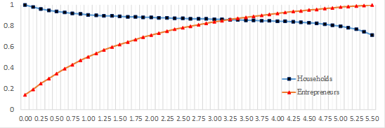
Additionally, as in Iacoviello (2005), entrepreneurs are subject to a collateral constraint such that the maximum amount of real credit depends on a proportion of the expected value of their net worth in the next period. This design allows linking the real variables with the financial ones through an extra constraint in their maximization problem, which also represents a financial friction. Therefore, there is a limit on their banking obligations considering their net worth, which depends on economic performance. In this way, the model captures the procyclicality of the banking system and, at the same time, the limitations faced by entrepreneurs when they require loans. For instance, the correlation between the GDP and the total financing to the non-financial private sector from commercial banks in Mexico is 0.35 from 2001 to 2019, such correlation can be appreciated in Figure 1. In addition, similar to Lama (2011), the model captures that the Mexican economy is a net debtor, so entrepreneurs have the capacity to borrow from abroad paying a risk premium3.

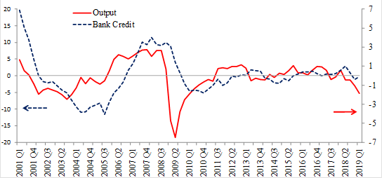
Note: Percentage deviations of its sample mean without trend.

Source: INEGI and Banco de Mexico.

Figure 1 Business and credit cycles.  

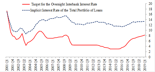
In the financial part of the model, consistent with Gerali et al. (2010), the banking sector is divided into other branches: a wholesale bank and retail banks. The wholesale bank exchanges financial assets between households and retail banks. This sector has no profits and requires accumulating bank capital to provide credit to the retail banks, obeying a balance sheet restriction. On the other hand, the retail banks receive credits from the wholesale bank and give them to the entrepreneurs, charging them a differential in the net interest rates. This branch has market power, which ensures that the loan rate is always higher than the deposit rate. In this way, the banking sector has different interest rates at the same time, one interest rate for deposits and another one for credits. Thus, the model is able to capture the spreads that there are in the Mexican banking system. In addition, the model incorporates a central bank that sets the deposits interest rate according to the inflation and the output gap, following a Taylor rule. Figure 2 displays the dynamics of these two net interest rates in Mexico4.

Finally, similar to Alpanda et al. (2018), the model includes two simplified reaction functions that represent the countercyclical macroprudential policies and respond to the credit-to-output ratio: a rule for CBCR and a rule for CLTVR. The particular specification of these rules allows an examination of an alternative situation where countercyclical rules are activated in comparison to a benchmark economy, which has constant bank capital requirements and fixed loan-to-value ratios.

Source: Banxico and CNBV.

Figure 2 Net nominal interest rates (%) 

2.1 Households

The representative household i chooses consumption ctH(i), hours worked nt(i) and real deposits dt(i) to maximize a lifetime utility function given by

E0t=0βHtlogctH(i)-χnt(i)1+σn1+σn

where E0 is the expectation operator, βH is the discount factor of the household sector, χ is a normalizing constant for labor, and σn is the inverse of the Frisch elasticity of labor supply. Households are subject to the following constraint

ctHi+dtiwtnt(i)+(1+rt-1d)dt-1(i)πt+trt

where wt is the real wage,Pt is the price of the consumption good, πt=Pt/Pt-1 denotes the gross inflation rate, rtd is the net nominal interest rate of deposits between the households and the wholesale bank, and trt are lump-sum profits received from the banking sector and the retailers (because households are the owners of these sectors). The first-order conditions are:

λtH=1ctH (1)

wt=χntσnλtH (2)

λtH=EtβH(1+rtd)λt+1Hπt+1 (3)

where λtH is the Lagrange multiplier of the budget constraint.

2.2 Entrepreneurs

The representative entrepreneur i chooses consumption ctE(i), labor input nt(i), loans from retailer banks lt(i), foreign debt lt*(i), and physical capital kt(i) to maximize a lifetime utility function given by

E0t=0βEtlogctE(i)

where βE is the discount factor for the business sector. Each entrepreneur is subject to the following constraints:

 yt(i)=Atkt-1(i)αnt(i)1-α (4)

ctEi+wtnti+ptkkti-1-δkt-1i +1+rt-1llt-1iπt+1+rt-1*lt-1*iπt*ptwyti+lti+lt*i (5)

(1+rtl)lt(i)mtEtpt+1kπt+11-δkt(i) (6)

Equation (4) represents the production constraint where the final good yt uses capital and labor as inputs. At denotes the stochastic process for total factor productivity and α is the capital share in the production function. Inequality (5) characterizes the budget constraint, where ptk is the real price of one unit of physical capital in terms of the consumption good, δ is the physical rate of depreciation, rtl is the net nominal interest rate of loans between entrepreneurs and retail banks, rt* is the net nominal interest rate of foreign debt, πt* is the external gross inflation rate, and ptw is the price at which they sell their products to retailers. Additionally, the external interest rate is

1+rt*=ς1+rUSlt*l*υ (7)

where ς represents the risk premium parameter, rUS is the net nominal interest rate of the US economy, and υ is the parameter that controls the elastic supply of foreign debt, as in Lama (2011). Assuming that the law of one price is satisfied, the equation that links both external and local inflations with the nominal exchange rate is:

πt*=πtet-1et. (8)

Inequality (6) represents the collateral constraint where the expected value of the collateralizable physical capital stock at period t must be high enough to guarantee that retail banks receive their payment. In this inequality, mt is the loan-to-value ratio, which can be interpreted as the amount of credit that banks make available to entrepreneurs for a given value of their physical capital stock5. As in Iacoviello (2005), βE<βH in order to guarantee the flow of financial assets. Indeed, this assumption implies a blinding collateral constraint at the steady-state, so entrepreneurs always request for the largest possible amount of loans. However, when there is uncertainty (i.e. stochastic productivity shocks), it may be the case that in some states of the economy entrepreneurs want to borrow less than their credit limit in order to buffer their consumption against adverse shocks or maybe they want to make default. Nevertheless, all exercises elaborated in this paper contemplate sufficiently small shocks in the economy such a way that the collateral constraint is always binding, and entrepreneurs pay their debts. In addition, productivity shocks are the drivers of the business cycle in the model6, so the stochastic process for the total factor productivity is

At=A(1-ρA)At-1ρAexpεtA. (9)

Consequently, after substituting (4) in (5), the first-order conditions of the entrepreneurs are:

λtE=1ctE (10)

wt=(1-α)ptwytnt (11)

λtE=EtβEλt+1E(1+rtl)πt+1+μt(1+rtl) (12)

λtE=EtβEλt+1E(1+rt*)πt+1* (13)

λtEptk=EtβEλt+1Ept+1k1-δ+αpt+1wyt+1kt+μtmt1-δpt+1kπt+1 (14)

where λtE is the Lagrange multiplier of the budget constraint and μt is the Lagrange multiplier of the collateral constraint. In the case that the collateral constraint is not binding at time t (i.e. μt=0), it is possible to find the standard uncovered interest rate parity condition using equations (8), (12), and (13), implying that

1+rtl=Et1+rt*et+1et.

Nevertheless, since the collateral constraint is always binding, it is not possible to derive a simple expression between the local and the external interest rates. This happens because local and external debts are not perfect substitutes, given that local debt is subject to a collateral constraint, while the foreign debt depends on the total amount of the external loan7.

2.3 Capital good producers

Capital good producers are used as a modeling device to derive a market price for physical capital, which determines the value of available collateral. They choose the optimal level of investment and follow a law of motion for physical capital accumulation that is subject to investment adjustment costs, as in Schmitt-Grohé and Uribe (2003). Following Gerali et al. (2010), capital good producers operate in a perfectly competitive market and use final consumption goods to produce capital goods. At time t, they buy it of final consumption goods and old undepreciated capital 1-δkt-1 from entrepreneurs. Next, they transform old undepreciated capital one-to-one into new capital while the transformation of the final goods is subject to the adjustment costs function υk2itit-1-12. Therefore, capital good producers choose investment iτ to maximize his lifetime profits function given by

Etτ=tβEτ-tλτEλtEpτk kτ-1-δkτ-1-iτ

s.t.      kτ=1-δkτ-1+1-υk2iτiτ-1-12iτ (15)

where υk is the intensity of the adjustment costs. The adjustment costs function is convex and equal to zero at the steady-state. Since entrepreneurs are the owners of this sector, future profits are again discounted using the entrepreneurs’ stochastic discount factor, so the first-order condition is:

1=ptk1-υk2itit-1-12-υkitit-1-1itit-1+βEEtλt+1EλtEpt+1kυkit+1it-1it+1it2. (16)

2.4 Banking system

As in Gerali et al. (2010), the banking sector in this model is divided into different branches, a wholesale branch and a loan branch. In this way, the model is able to separate the optimal decision on bank capital, according to the bank capital requirements, and the optimal spread that the bank system charges when setting interest rates, generating a differential between the deposit rate and the loan rate.

2.4.1 Wholesale bank

Wholesale bank acts as an intermediary between households and retail banks, operates in a perfectly competitive market and has to obey a balance sheet restriction

dt+Capt=lt (17)

where lt are the real loans from retail banks,dt are the real deposits from households, and Capt is the bank equity or bank capital (the real net worth of the bank system). Deposits and bank capital are perfect substitutes from the point of view of the balance sheet to offer credits. However, bank capital is accumulated according to a dividend policy, where the profits of the entire banking system are distributed between the creation of new bank capital and the payment of dividends. This policy is consistent with the following equation

πtCapt=1-δcapCapt-1+ωψt-1 (18)

where δcap represents the percentage of expenses destined to manage the bank capital, ψt are the profits of the entire banking system, and ω is the proportion of profits destined to accumulate new capital. Neither the wholesale bank nor the retail banks have control over this dividend rule, so bank capital is an exogenous variable to them.

Subject to the balance sheet restriction, the wholesale bank chooses loans and deposits at time t to maximize the cash flow defined as

rtwlt-rtddt-υcap2Captlt-γt2Capt

where rtw is the net interest rate of loans between the wholesale bank and retail banks, so rtwlt represents the income that the wholesale bank receives from retail banks because of the sale of credits8. On the other hand, the other two terms represent the wholesale bank expenditures, where the former represents the payment to households for the deposits and the latter represents the cost of the wholesale activity related to the capital position of the bank. In other words, the last term represents the cost that the wholesale bank has to pay to satisfy the banking regulation. In particular, the wholesale bank pays a quadratic cost whenever the capital-to-assets ratio Capt/lt moves away from the target value γt, parameterized by υcap>0. Since dt=lt-Capt, the unique first-order condition with respect to lt is

rtw=rtd-υcapCaptlt-γtCaptlt2 (19)

where rw is equal to rd at the steady state because the wholesale bank obeys the banking regulation.

2.4.2 Retail banks

Retail banks are responsible for introducing market power that allows them to adjust rates on loans to be greater than the deposit rates. Following Gerali et al. (2010), they are monopolistic competitors on the loan markets, infinitely lived, and of measure one. At time t, they obtain credits from the wholesale bank at rate rtw, differentiate them, and resell them to entrepreneurs. Also, each retail bank faces quadratic adjustment costs à la Rotemberg in order to introduce sticky interest rates, parameterized by υl. Thus, the representative retail bank j solves the following problem

maxrτljEtτ=tβHτ-tλτHλtHrτljlτj-rτwlτj-υl2rτljrτ-1lj-12rτllτ

s.t.     lτj =rτljrτl-ϵlτ.

Households are the owners of this sector, so future profits are again discounted using the households’ stochastic discount factor. Therefore, the first-order condition is

1-ϵ+ϵrtwrtl-υlrtlrt-1l-1rtlrt-1l+βHEtλt+1HλtHυlrt+1lrtl-1rt+1lrtl2lt+1lt=0. (20)

The price elasticity of demand for lτj is ϵ>1, which defines the value of the markup that retail banks charge when setting interest rates and, consequently, the value of the spread between the monetary policy rate and the retail loan rate. Thus, the markup can be defined as

rl=ϵϵ-1 rw

at the steady-state, implying that rl>rw, so the banking system always generates positive profits.

2.5 Retailers

Retailers incorporate sticky prices into the model. According to Leith and Liu (2016), they are monopolistic competitors, infinitely lived, and of measure one. Each retailer buys yt from entrepreneurs at price ptw in a competitive market, differentiates the goods into yt(j), and sells them at the nominal price Pt(j). Also, each retailer faces a quadratic cost of adjusting nominal prices, which depend on the ratio between the new reset price Pt(j) and the one set during the previous period, Pt-1(j). As well as with the banking sector, households are the owners of the retail sector so future profits are again discounted using the households’ stochastic discount factor. As a result, the representative retailer solves the following problem

maxPt(j)Ets=0βHsλt+sHλtHPt+s(j)Pt+s-pt+swyt+s(j)-θ2Pt+s(j)Pt+s-1(j)-12yt+s

s.t.     yt+s(j)=Pt+s(j)Pt+s-ξyt+s

where θ determines the rigidity degree and ξ>1 describes the Dixit-Stiglitz elasticity of substitution among goods. Thus, the first-order condition is

θπt-1πt=(1-ξ)+ξptw+βHθEtλt+1HλtHπt+1-1πt+1yt+1yt (21)

2.6 Monetary and macroprudential policies

As in Gerali et al. (2010), the central bank set the interest rate rtd according to the equation

1+rtd=1+rt-1dϕR1+rd-πtπϕπytyt-1ϕy(1-ϕR) (22)

where ϕR, ϕπ, and ϕy characterize the weights assigned to the interest rate, inflation and output gap stabilization, respectively. The countercyclical macroprudential rules are defined as

γt=γ-ltyt/lyϕγ (23)

mt=m-ly/ltytϕm (24)

where ϕγ and ϕm are the weights assigned to the credit-to-output ratio in the macroprudential tools, so these parameters measure the sensitivity of each rule to the deviations of the credit-to-output ratio with respect to its long-term equilibrium.

In this paper, two main cases are analyzed according to the values of ϕγ and ϕm, and used to study the effects of introducing macroprudential regulation on social welfare. The first case is when the model has ϕγ=ϕm=0, implying that CBCR and CLTVR are constant. This situation represents a benchmark economy where there is no countercyclical regulation, so the wholesale bank acts according to fixed banking regulation, and entrepreneurs are restricted by a constant loan-to-value ratio. On the other hand, there is a second case where ϕγ and ϕm are positive, implying that macroprudential tools are activated. Thus, in the situation where ltyt>ly, the countercyclical tool for bank capital requirements will increase the bank capital, so γt>γ- in order to buffer the total debt growth. Meanwhile, the countercyclical tool for the loan-to-value ratios will decrease the entrepreneurs’ credit through their collateral constraint, so mt<m-.

2.7 Equilibrium

The profits of the entire banking system are defined as

ψt=rtllt-rtddt-υcap2Captlt-γt2Capt-υl2rtlrt-1l-12rtllt (25)

the household sector is subject to the constraint

ctH+dt=wtnt+1+rt-1ddt-1πt+1-ωψt+yt1-ptw-θ2πt-12 (26)

where the lump-sum profits from the banking sector and the retailers are now well defined9, and the total consumption is

ct=ctH+ctE. (27)

Given that the model includes the households’ budget constraint, an equilibrium condition in the final good market is redundant. However, with equations (5), (18), (25), (26), and (27) at the steady state, it is possible to derive an expression of this equilibrium condition, which is equal to

y=c+i+δcapCap+r*l*.

Therefore, the equilibrium for this model is a set of sequences for the quantities {ctH,ctE,ct,it,kt,nt,yt,dt,lt,lt*,Capt,ψt}t=0 together with the sequence of prices {πt,ptk,ptw,wt, rtd,rtw,rtl,rt*,et}t=0 and values {At,γt,mt,λtH,λtE,μt}t=0 such that satisfy equations (1) to (27) with the sequence of shocks {εtA}t=0, given A0,k0,d0,l0,l0*,Cap0,r0d, r0w,r0l,r0*, and e0. In the absent of shocks, the model has a unique stationary equilibrium, all rigidities disappear, and the entrepreneurs hit the borrowing constraint.

3. Calibration

The set of parameters is calibrated to match the main features of the Mexican data from 2001 Q1 to 2019 Q1 (in quarterly terms), considering the model equations at the steady-state.

The model integrates standard values for ρA,δ, and α, following Aguiar and Gopinath (2007), and García-Verdú (2005). The elasticity of substitution is 1.25 and the degree of nominal price rigidity is defined according to Leith and Liu (2016), where θ=(ξ-1)φ(1-φ)(1-φβH) and φ is the probability of not changing prices each quarter. So, φ=0.783 as in Ramos-Francia and Torres (2006), implying that θ=3.945. The investment adjustment cost is equal to 0.2 considering Brzoza-Brzezina and Makarski (2011). For the labor parameters, σn=0.97 while χ is adjusted to obtain a consistent fraction of full-time working hours, as in Adame et al. 2016). The households’ discount factor is calibrated using equation (3) and the net real interest rate, which is equal to 0.516% per quarter, thus βH=0.995 (Banxico, 2017b). The banking system markup is adjusted by equations (19) and (20), and the implicit interest rate, which includes all the banking sector credits in Mexico (CNBV, 2018), so ϵ=1.937. In addition, βE is consistent with this implicit interest rate and with a positive μ, thus βE=0.87.

For the reaction functions that represent the monetary and macroprudential policies, the model incorporates the current banking regulation and the observed monetary policy reaction in Mexico. Thus, γ- is equal to 11% according to CESF (2019) and m- is equal to 64.4% by CESF (2013) and CNBV (2012). Following Ramos-Francia and Torres (2005), ϕR, ϕπ, and ϕy are equal to 0.58, 1.75, and 0.56, respectively. Since ϕγ and ϕm measure the sensitivity of each countercyclical policy, they are equal to zero to reproduce the benchmark economy. Furthermore, δcap=0.1, ω=0.591, υcap=10, and υl=3 to characterize the banking system dynamics, as in Gerali et al. (2010)10.

According to Lama (2011), for the parameters associated with the foreign debt, equation (7) incorporates a highly elastic supply of funds because its purpose is to induce stationarity in the model rather than to capture the behavior of the risk premium, so υ is small. On the other hand, the value of rUS is consistent with the U.S. policy interest rate, and ς is found using equations (7) and (13).

Figure 3 shows the dynamic cross‐correlations for the Mexican data and the model. Two cases are displayed: a model without rigidities and a benchmark economy where all frictions are activated. Both cases only consider productivity shocks without macroprudential policy. In the case without frictions, the model does not capture correctly the empirical correlation. In particular, the investment dynamics are distant from the confidence interval for several correlations. On the contrary, the benchmark economy performs better results as it gets closer to the data, especially for t equal to -1, 0, and 1. However, the benchmark economy incorporates a more persistent correlation between the variables in comparison to the empirical point estimates11.

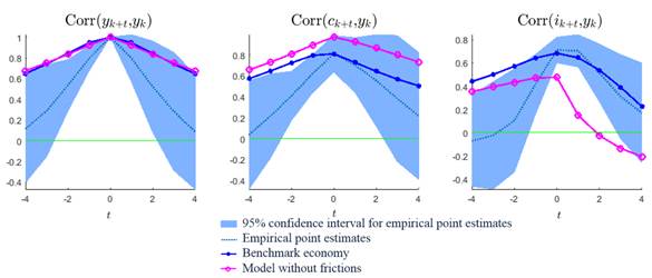
Note: dynamic cross‐correlations are computed with a simulation of 10,000 draws where the first 10% of the sample was eliminated. Confidence intervals are consistent with the methodology of Christiano et al. (2014).

Source: Own elaboration.

Figure 3 Dynamic cross‐correlations.  

4. Welfare Analysis

The next step is to find numerically the adequate reaction that the macroprudential rules must have. Thus, it is necessary to test the possible values that the parameters ϕm and ϕγ can take, verifying which one of them improves or damages the welfare of each agent in comparison to the benchmark economy. To find the best pair (ϕm,ϕγ), a mesh is constructed where each direction represents a parameter that goes from 0 to a maximum value in such a way that it covers many values between those numbers. The maximum value is found until the Blanchard-Kahn conditions are no longer satisfied (i.e. when the model does not have a stable solution). This mesh has a sufficiently large number of pairs (ϕm,ϕγ) that are evaluated into the model using stochastic simulations of productivity shocks. After evaluating each pair, a welfare assessment is elaborated for households and entrepreneurs, separately. The welfare estimation is based on a second-order approximation to the households’ and entrepreneurs’ period utility functions around the deterministic steady state, following the process developed by Schmitt-Grohé and Uribe (2004)12.

The households’ welfare is calculated as follows:

1. Since the present discount value of the households’ utility function is

UtH=Ets=0βHsVt+sH= Ets=0βHslogct+sH-χnt+s1+σn1+σn

where VtH=VH(ctH,nt) is the period utility function, the second-order approximation to VtH around the deterministic steady state is

VHctH,ntVHcH,n+VcHHcH,nctH-cH+VnHcH,nnt-n+12VcHcHHcH,nctH-cH2+VcHnHcH,nctH-cHnt-n+12VnnHcH,nnt-n2+O(E3)

2. Ignoring O3, the residual term, the approximation can be rewritten as

VHctH,ntlogcH-χn1+σn1+σn+ctH-cHcH-χnσnnt-n-12ctH-cH2cH2-12χσnnσn-1nt-n2

Therefore, the expected infinite discounted sum of the period utilities is

UtH Ets=0βHslogcH-χn1+σn1+σn+ctH-cHcH-χnσnnt-n-12ctH-cH2cH2-12χσnnσn-1nt-n2

=11-βHlogcH-χn1+σn1+σn+EtctH-cHcH-Etχnσnnt-n-Et12ctH-cH2cH2-Et12χσnnσn-1nt-n2

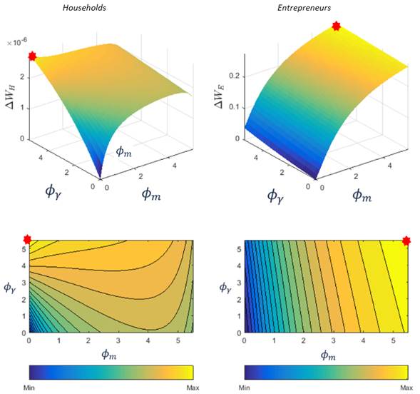
Note: The red star represents the pair that maximizes the welfare of each sector, which can be identified by being close to the yellow color and far from the blue color. Additionally, the contour lines are added to observe more details about the behavior of the percent change of welfare.

Source: Own elaboration.

Figure 4 Welfare evaluation.  

3. Since EtctH=cH, Etnt=n, and EtctH-cH2=VarctH-cH-EtctH-cH2, the households’ welfare can be written as

WtH=11-βHlogcH-χn1+σn1+σn-12VarctHcH2-12χσnnσn-1Varnt

Therefore, to compute the households’ welfare under different policy rules, it is only necessary to calculate the variances of consumption and labor across simulations of productivity shocks and plug them into WtH. In the same way, after several steps, the entrepreneurs’ welfare is

WtE=11-βElogcE-12VarctEcE2.

Figure 4 shows the welfare’s percent change for each agent, using each pair (ϕm,ϕγ) of the mesh. In the charts, it can be appreciated that the implementation of CBCR and CLTVR, represented by positive values of ϕγ and ϕm, has positive effects on welfare, especially for CBCR. In particular, the best macroprudential regulation for households is ϕm,ϕγ=(0,5.5), while entrepreneurs prefer ϕm,ϕγ=(5.5,5.5). In terms of the standard compensating consumption variation, these pairs represent a gain in consumption of 3.42×(10-8)% and 0.018% in comparison to the benchmark economy, respectively.

5. Results

According to the previous findings, it is better to use ϕγ=5.5 for both agents, but there is a discrepancy regarding the value of ϕm. Households prefer a value equal to zero while entrepreneurs reach their maximum welfare gain with a value of 5.5. This means that there is a set of macroprudential rules such that ϕm,ϕγ=ϕ,5.5, with ϕϵ&#091;0,5.5&#093;, which generates a welfare improvement for the economy in comparison to the benchmark situation. However, there is a trade-off between the households’ welfare and the entrepreneurs’ welfare on these rules. Hence, this paper analyzes a particular case where both agents receive the same improvement in terms of their own percent change of welfare. To find this case, it is necessary to normalize the percent change of welfare for each agent in order to make them comparable. So, when ϕγ=5.5 and ϕϵ&#091;0,5.5&#093;, each welfare’s percent change is divided by the maximum possible value in such a way that the best pair (ϕm,ϕγ) of each agent is equal to 1 (and equal to 0 for the benchmark economy because there is no improvement in this case). Therefore, the pair ϕm,ϕγ=3.25,5.5 generates the same percentage improvement for both agents in comparison to the economy without macroprudential rules. Figure 5 displays these results.

Source: Own elaboration.

Figure 5 Welfare (percent change, normalized)  

As a result, now it is possible to analyze how CBCR and CLTVR affect the economy and verify whether these rules meeting their goals of banking stability. This means that these instruments should smooth a credit boom (or a credit crunch) and avoid a situation where the economy is indebted beyond (or below) its long-term equilibrium.

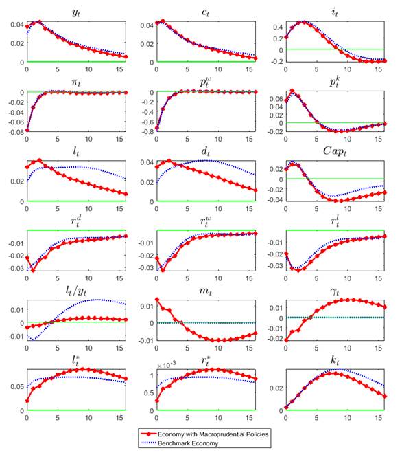
Note: All rates are shown as absolute deviations from steady state, expressed in percentage points. All others variables are percentage deviations from steady state.

Source: Own elaboration.

Figure 6 Impulse-response functions.  

Figure 6 shows the impulse response functions of the main model variables following a positive productivity shock for two cases: the current banking regulation (i.e. the benchmark economy) and the alternative situation where the countercyclical tools are activated, ϕm,ϕγ=3.25,5.5. For the benchmark economy (the blue dotted line), the impulse responses are qualitatively similar to Gerali et al. (2010) because the transmission mechanisms are comparable. Investment is boosted both by the technological improvement and by a particularly eased access to credit. Thus, the accumulation of physical capital pushes asset prices up, implying that borrowers benefit from the wider access to credit that higher collateral value affords. Additionally, the downward pressure on prices induces a monetary policy rate cut and there is a delay in the propagation of the monetary policy rate to the bank lending rate. Therefore, this improvement in credit conditions (given by the collateral constraint and the reduction in interest rates) boosts the real activity as well as the leverage, for both local and foreign credits. This effect allows entrepreneurs to expand investment further, which in turn induces a higher price of capital and hence higher technological improvement, illustrating the financial acceleration mechanism that the model has.

On the other hand, in the alternative situation where macroprudential policies are activated (the red circled line), CBCR and CLTVR are successful in keeping the credit-to-output ratio according to its long-term equilibrium. Initially, during the first periods, CBCR and CLTVR facilitate the credit conditions to take advantage of the productivity shock. However, periods later, these rules restrict credit conditions to avoid a high credit-to-output ratio once the productivity shock diminishes. In comparison to the benchmark economy, the credit-to-output ratio falls quickly and mitigates the adverse effects of a bust afterward where the economy is heavily indebted. The intuition behind these results is the following: CBCR are efficient in keeping a stable credit-to-output ratio because they give incentives to households to save depending on the business cycle, while CLTVR motivate entrepreneurs to borrow according to the productivity shocks.

As a result, high credit deviations that could generate a banking crunch, which in turn could create an economic crisis, are not possible because the credit-to-output ratio always goes hand in hand with macroeconomic fundamentals. For instance, consider the entrepreneurs’ perspective under a positive productivity shock. Under the benchmark situation, in the collateral constraint at time t, entrepreneurs can expand their production and loans since the shock boosts the expectation of their net worth Etpt+1kπt+11-δkt. However, this expectation is different from the true realized value because, when the collateral constraint interacts with the general equilibrium, it is not possible to support such expansion (banks and households cannot afford such increase). Thus, entrepreneurs end up with a higher level of loans that affect them throughout the convergence path (i.e. affects their welfare), making a riskier bank system. On the other hand, when there are countercyclical tools, mt avoids a large deviation of credits only when the productivity shock is absent, implying that there is a limit in the credit cycle only when it is not justified by productivity shocks, which are the macroeconomic fundamentals in this model. Hence, countercyclical tools evade the negative effects of having an economy with high levels of credit.

Regarding the creation of credit bubbles or high credit deviations, some additional clarifications must be considered. A credit bubble is a positive deviation in the relationship between credit and economic activity, and there are several methodologies that quantify it. For instance, Dell’Ariccia et al. (2012) provide a definition using the credit-to-output ratio that can be applied to a sample of 170 countries to identify the stylized facts that describe credit booms13. However, for the Mexican case and the BIS’ recommendation about the countercyclical capital buffers, a credit bubble is characterized when the credit-to-output ratio deviates positively from its trend by two percent. Therefore, an additional exercise is elaborated to show how the credit-to-output ratio dynamics change over time according to different banking regulations. Given a random path of productivity shocks, two simulated credit-to-output ratios are generated over time, one for the benchmark economy and another one for the alternative case. For the benchmark economy, there is a probability of 36.07% that the credit-to-output ratio excess the 2% threshold, which is consistent with the empirical behavior of the credit-output ratio deviations from its long-term trend (Banxico, 2017). In this case, the model produces credit bubbles because of the collateral constraint. This restriction specifies that the current value of the entrepreneurs’ debt grows according to the expected value of their collateralizable physical capital stock, which in turn depends on the contemporary investment. Therefore, when there is a positive productivity shock, there is an increase in the investment that produces a boost in the capital stock, which allows a persistent debt level and a positive credit-to-output ratio deviation for several periods. However, for the counterfactual case, CBCR and CLTVR do not tolerate significant credit-to-output ratio deviations, thus the creation of credit bubbles is very unlikely. In fact, its probability is equal to 0.6% in the model simulation. This exercise is displayed in Figure 7. Note that CBCR and CLTVR neither tolerate credit turndowns, showing their ability to deal with significant negative shocks, like the current COVID‑19 pandemic.

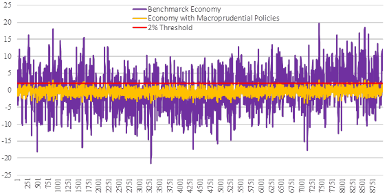
Note: Percentage deviations of its steady states. The exercise is computed with a simulation of 10,000 draws where the first 10% of the sample was eliminated.

Source: Own elaboration.

Figure 7 Credit-to-output ratio simulations.  

As a result, CBCR and CLTVR are able to attenuate credit-to-output volatility because of two reasons. First, CBCR allow a persistent debt level only if there is a high accumulation of bank capital requirements, something that it is not possible because affects the banking sector’s profitability. And second, CLTVR mitigate entrepreneurs’ ability to preserve a high amount of loans because now the collateral constraint contemplates the loan-to-value ratio dynamics, which attenuates the effect of the expected value of the collateralizable physical capital stock over their debt14.

6. Policy Issues

There are some difficulties associated with the performance of time-varying macroprudential policies. Their implementation is not easy because of the need for detailed data about the banking sector and the real activity, the appropriate institutions, and the right policy rules to control the credit flows in the economy. However, despite all these complications, the use of the macroprudential tools in the Mexican economy is possible and several facts support this statement. In particular, the COVID-19 outbreak has accelerated the need to implement this new regulation, making this research highly helpful for policymakers during this pandemic.

The IMF has highlighted the Mexican progress to formally establish a financial stability committee to coordinate relevant information about the economy’s state between different regulatory agencies, laying the groundwork for the implementation of macroprudential policies (Carrière-Swallow et al. 2016). In 2010, Mexico created the Financial System Stability Council (CESF, for its initials in Spanish) with the objective to promote financial stability, avoiding interruptions, or substantial alterations in the functioning of the financial system and, where appropriate, minimize its impact when these take place (CESF, 2019)15. In particular, if any risk is identified in the financial system, the Council has the faculty to elaborate recommendations and act as a forum for policy coordination. Therefore, any type of macroprudential policy has to be approved and executed by this Council, considering at all times its congruence and coordination with other macroeconomic policies, especially with the fiscal and the monetary stance. As Guzman (2013) points out, monetary and macroprudential policies must work in a complementary way toward the achievement of their objectives and mutually strengthen one another.

On the other hand, it is possible to identify a situation when the economy or a specific sector is indebted beyond its capacity, considering that the main features of each loan in the Mexican banking system are measurable through the databases available for the Council16. For instance, if a response from the Council is required, one solution is to use the countercyclical tool for loan-to-value ratios that will decrease the ability of debtors to have high debt levels. This solution can be represented in practice by any regulation that changes the debt amount or the conditions offered by each bank, like collateral requirements, commissions, or other types of restrictions. Empirically, loan-to-value ratios are the most used tool according to Akinci and Olmstead-Rumsey (2015). They find that loan-to-value ratios are effective instruments for controlling credit levels, both for advanced and for emerging economies, especially for the housing sector.

Another solution that the Council can implement is the use of countercyclical bank capital requirements, which means changing the minimum capital requirements according to the business cycle without any limitations. Note that the rule of CBCR is different from countercyclical capital buffers (CCB), which is another instrument proposed by the Basel Committee on Banking Supervision among its members. CCB establish that countercyclical reserves must be created only during boom phases of the economic cycle and used during the downward phases. These capital reverses will react to credit-to-output ratio deviations in such a way that banks should only start to build up CCB when this indicator is greater than two percent (BIS, 2018). Therefore, the modeling of CCB is complicated because this rule reacts asymmetrically to the credit-to-output ratio considering a specific threshold. As a result, the proposed model in this paper can be a prototype to analyze CCB in a more complex setting17. For now, CBCR have already shown that they are effective in meeting their goals of banking stability and welfare improvement. Meanwhile, more research is needed to know the effects of implementing CCB. For instance, Carstens (2016) shows how CCB are particularly challenging in an emerging economy with low levels of financial deepening, mainly because the credit demand will grow beyond its current level, implying that the activation of CCB should not be guided exclusively by the credit-to-output ratio. Thus, CCB should be activated only when credit growth is driven by “supply factors” 18.

Amid the COVID-19 outbreak and related expected economic downturn, many emerging economies are dealing with serious financial distress, requiring new instruments beyond the conventional fiscal and monetary policies. For the Mexican case, on 04/09/2020, the National Commission of Banks and Securities authorized banks to use their capital conservation supplement to help their balance sheet19. In terms of the model, this regulation implies that γt=8.5% for one year. On the other hand, on 04/21/2020, Banxico simultaneously announced corporate bond and government bond purchases, as well as a reduction in the interest rate20. On 07/31/2020, Banxico allowed banks to carry out financial leasing and factoring operations with small businesses with the resources derived from the facilities provided by the same central bank. Also, Banxico authorized the same kind of regulation to help the recovery of auto loans and mortgage credits, facilitating credits to individuals21. In terms of the model, this regulation implies an increase in mt but its magnitude and duration will depend on how banks use the loan-to-value ratios. Possibly, in the near future, more instruments can be implemented not only in Mexico but also in other emerging economies. So more research will be required to understand their effects and how useful are mitigating the pandemic shock. Meanwhile, given the results in Section 4 and 5, it is clear that these macroprudential policies have the potential to moderate the COVID-19 outbreak.

7. Conclusions

This paper is the first attempt to analyze the welfare implications of countercyclical bank capital requirements (CBCR) and countercyclical loan-to-value ratios (CLTVR) in Mexico using a DSGE model, with the purpose to be useful in the public debate about macroprudential regulation. Using total factor productivity shocks and a second-order approximation of the utility functions, CBCR and CLTVR show their capacity to improve the Mexican welfare compared to a situation where there is no countercyclical regulation. In particular, CBCR and CLTVR facilitate or restrict credit conditions in order to follow the productivity shocks that hit the Mexican economy. This means that these rules are efficient giving incentives to savers and debtors to save and to get into debt only along with the productivity shocks, implying that it is not possible a situation where economic agents get an additional or less credit over their fundamentals. Therefore, the formation of credit bubbles that could generate an eventual banking crunch, which in turn could create an economic crisis, is not possible because the credit-to-output ratio always goes hand in hand with macroeconomic conditions. Also, in the case of a severe turndown of the economy, these rules show to be effective in facilitating loans to the business sector, independently of the reaction of the fiscal and monetary authority. Even though there are some difficulties associated with their use, nowadays there are sufficient conditions to use macroprudential tools. Results suggest that a countercyclical intervention in Mexico may well be needed in the near future and exploring alternative macroprudential policy responses is an interesting agenda for upcoming research.

In addition, results are useful to justify the implementation of time-varying macroprudential policies in Mexico. There are sufficient conditions to use CBCR and CLTVR since the legal arrangements, institutional design, and economic information are capable to allow an effective execution of these rules. CBCR and CLTVR represent a useful guide to recognizing the important variables and the main effects that policymakers should consider in real life. In particular, they should preserve the credit-to-output ratio according to its long-term equilibrium and look out its fluctuations according to the economic activity. Also, they should observe the accumulation of bank capital in order to avoid possible financial difficulties, as well as guarantee that there is an adequate debt level in the economy. Given the growth of the Mexican financial system in recent years, it is necessary to use additional measures that keep banking stability in the country, and macroprudential regulation can achieve this objective, especially during the COVID-19 outbreak.

References

Adame, F., Carrillo, J., Roldan-Peña, J., and Zerecero, M. (2016). Financial considerations in a small open economy model for Mexico. Mimeo. [ Links ]

Agenor, P., and Jia, P. (2020). Capital Controls and Welfare with Cross-Border Bank Capital Flows. Journal of Macroeconomics, Volume 65, September 2020, 103220. https://doi.org/10.1016/j.jmacro.2020.103220Links ]

Aguiar, M., and Gopinath, G. (2007). Emerging market business cycles: the cycle is the trend. Journal of Political Economy, 115, 69-102. https://doi.org/10.1086/511283Links ]

Akinci, O., and Olmstead-Rumsey, J. (2015). How Effective are Macroprudential Policies? An Empirical Investigation. International Finance Discussion Papers - Board of Governors of the Federal Reserve System, No. 1136. https://doi.org/10.17016/ifdp.2015.1136Links ]

Alpanda, S., Cateau, G., and Meh, C. (2018). A Policy Model to Analyze Macroprudential Regulations and Monetary Policy. Canadian Journal of Economics, vol. 51, issue 3, 828-863. https://doi.org/10.1111/caje.12339Links ]

Banco de México. (2010). Reporte sobre el Sistema Financiero. https://www.banxico.org.mxLinks ]

Banco de México. (2013). Reporte sobre el Sistema Financiero. https://www.banxico.org.mx Links ]

Banco de México. (2016). Reporte sobre el Sistema Financiero. https://www.banxico.org.mxLinks ]

Banco de México. (2017a). Reporte sobre el Sistema Financiero. https://www.banxico.org.mxLinks ]

Banco de México. (2017b). Principales Activos y Pasivos de la Banca Comercial. https://www.banxico.org.mx/SieInternet/Links ]

Bank for International Settlements (BIS). (2018). Countercyclical capital buffer (CCyB). https://www.bis.org/bcbs/ccyb/Links ]

Basel Committee on Banking Supervision (BCBS). (2009). Strengthening the resilience of the banking sector. Bank for International Settlements, December 2009. https://www.bis.org/publ/bcbs164.htmLinks ]

Binning, A., and Maih, J. (2017). Modelling Occasionally Binding Constraints Using Regime-Switching. Norges Bank Research, No. 23. https://doi.org/10.2139/ssrn.3073753Links ]

Blanchard, Oliver, Dell’Ariccia, G., and Mauro, P. (2013) Rethinking Macro Policy II: Getting Granular. IMF Staff Discussion Note. https://www.imf.org/external/pubs/ft/sdn/2013/sdn1303.pdfLinks ]

Blundell-Wignall, A. , and Roule, C. (2014). Macro-prudential policy, bank systemic risk and capital controls. OECD Journal: Financial Market Trends 2014. https://doi.org/10.1787/fmt-2013-5jzb2rhkhks4Links ]

Bodenstein, M., Guerrieri, L., and LaBriola, J. (2014). Macroeconomic Policy Games. Finance and Economics Discussion Series 2014-87, Board of Governors of the Federal Reserve System. https://doi.org/10.17016/feds.2014.87Links ]

Brzoza-Brzezina, M. and Makarski, K. (2011). Credit crunch in a small open economy. Journal of International Money and Finance, 30,1406-1428. https://doi.org/10.1016/j.jimonfin.2011.07.010Links ]

Carrière-Swallow, Y., Jácome, L., Magud, N., and Werner, A. (2016). Central Banking in Latin America: The Way Forward. Carrière-Swallow, Y., Faruqee, H., Jácome, L., and Srinivasan, K., Challenges for Central Banking - Perspectives from Latin America, 41-79, International Monetary Fund. https://www.imf.org/en/Publications/WP/Issues/2016/12/31/Central-Banking-in-Latin-America-The-Way-Forward-44317 Links ]

Carrillo, J., Mendoza, E., Nuguer, V., and Roldán-Peña, J. (2020). Tight Money-Tight Credit: Tinbergen’s Rule and Strategic Interaction in the Conduct of Monetary and Financial Policies. American Economic Journal (Forthcoming). https://www.aeaweb.org/articles?id=10.1257/mac.20180321&&from=fLinks ]

Carstens, A. (2016). Micro-data as a Key Input to Designing Macro-prudential Policy: The Mexican Experience. Remarks at the Eighth European Central Bank Conference on Statistics. https://www.ecb.europa.eu/pub/conferences/shared/pdf/160705_8th_stats_conference/Carstens.pdfLinks ]

Chang, C., Liu, Z., and Spiegel, M. (2015). Capital Controls and Optimal Chinese Monetary Policy. Federal Reserve Bank of San Francisco, Working Paper 2012-13. https://doi.org/10.24148/wp2012-13Links ]

Christiano, Lawrence J., Motto, R., and Rostagno, M. (2014). Risk Shocks. American Economic Review, 104 (1): 27-65. https://doi.org/10.1257/aer.104.1.27Links ]

Comisión Nacional Bancaria y de Valores (CNBV). (2012). Encuesta Nacional de Competitividad, Fuentes de Financiamiento y Uso de Servicios Financieros de las Empresas, Reporte de Resultados. https://www.cnbv.gob.mx/CNBV/Estudios-de-la-CNBV/Encuesta%20Empresas/Resultados_Encuesta_Nacional_Competitividad.pdfLinks ]

Comisión Nacional Bancaria y de Valores (CNBV). (2018). Indicadores financieros: históricos (series desde diciembre 2000). http://portafoliodeinformacion.cnbv.gob.mx/bm1/Paginas/infosituacion.aspxLinks ]

Consejo de Estabilidad del Sistema Financiero (CESF). (2013). Informe anual. https://www.gob.mx/ipab/articulos/consejo-de-estabilidad-del-sistema-financiero-en-mexicoLinks ]

Consejo de Estabilidad del Sistema Financiero (CESF). (2019). Informe anual. https://www.gob.mx/ipab/articulos/consejo-de-estabilidad-del-sistema-financiero-en-mexicoLinks ]

Garcia-Barragan, F. and Liu, G. (2018). Welfare analysis of bank capital requirements with endogenous default. Economic Modelling. https://doi.org/10.1016/j.econmod.2018.03.002Links ]

Garcia-Cicco, J., Kirchner, M., Carrillo, J., Rodriguez, D., Perez, F., Gondo, R., Montoro, C., and Chang, R. (2017). Financial and real shocks and the effectiveness of monetary and macroprudential policies in Latin American countries. BIS Working Papers No 668, Monetary and Economic Department. https://www.bis.org/publ/work668.pdfLinks ]

Garcia-Verdu, R. (2005). Factor shares from household survey data. Banco de Mexico, Working Paper 2005-05. https://doi.org/10.36095/banxico/di.2005.05Links ]

Gerali, A., Neri, S., Sessa, L., and Signoretti, F. (2010). Credit and Banking in a DSGE Model of the Euro Area. Journal of Money, Credit and Banking, Blackwell Publishing, vol. 42, 107-141. https://doi.org/10.1111/j.1538-4616.2010.00331.xLinks ]

Guerrieri, L., and Iacoviello, M. (2015). OccBin: A toolkit for solving dynamic models with occasionally binding constriants easily. Journal of Monetary Economics, 70, 22-38. https://doi.org/10.1016/j.jmoneco.2014.08.005Links ]

Guzman Calafell, J. (2013). Challenges for macroprudential policy and the Mexican case. Remarks at the panel on Macroprudential policies for securing financial stability in a volatile external liquidity environment, Fifth Summit Meeting of Central Banks on Inflation Targeting, Santiago de Chile, 15-16 November 2013. https://www.banxico.org.mx/publicaciones-y-prensa/discursos/discursos-junta-gobierno-pala.htmlLinks ]

Hartley, J., and Rebucci, A. (2020) An Event Study of COVID-19 Central Bank Quantitative Easing in Advanced and Emerging Economies. NBER Working Paper No. 27339, June 2020. https://doi.org/10.3386/w27339Links ]

Iacoviello, M. (2005). House Prices, Borrowing Constraints and Monetary Policy in the Business Cycle. American Economic Review, Vol. 95(3), pp. 739-764. https://doi.org/10.1257/0002828054201477Links ]

Laeven, L., and Valencia, F. (2012). Systemic Banking Crises Database: An Update. IMF Working Paper 2012-163. https://www.imf.org/external/pubs/ft/wp/2012/wp12163.pdfLinks ]

Lama, R. (2011). Accounting for output drops in Latin America. Review of Economic Dynamic, 14, 295-316. https://doi.org/10.1016/j.red.2010.12.001Links ]

Leith, C., and Liu, D. (2016). The inflation bias under Calvo and Rotemberg pricing. Journay of Economic Dynamics & Control, 73, 283-297. https://doi.org/10.1016/j.jedc.2016.09.002Links ]

Mier-y-Teran, A. (2012). Bank Competition and the Transmission of Monetary Policy. Manuscript, UCLA. https://blogs.worldbank.org/sites/default/files/allaboutfinance/bank_competition.pdfLinks ]

Ramos-Francia, M., and Torres, A. (2005). Reducción de la Inflación a Través de un Esquema de Objetivos de Inflación: La Experiencia Mexicana. Banco de Mexico, Working Paper 2005-01. https://doi.org/10.36095/banxico/di.2017.12Links ]

Ramos-Francia, Manuel and Torres, A. (2006). Inflation Dynamics in Mexico: A Characterization Using the New Phillips Curve. Banco de Mexico, Working Paper 2006-15. https://doi.org/10.36095/banxico/di.2006.15Links ]

Roldán-Peña, J., Torres-Ferro, M., and Torres, A. (2016). Financial Stability Objectives: Drivers of Gains from Coordinating Monetary and Macroprudential Policies. Banco de Mexico, Working Paper 2017-22. https://doi.org/10.36095/banxico/di.2017.22Links ]

Sámano, D. (2011). In the quest for macroprudential policy tools. Central Bank Award Rodrigo Gómez, CEMLA, 2011. https://www.cemla.org/PDF/premiobc/pub-lib-premio2011.pdfLinks ]

Schmitt-Grohé, S., and Uribe, M. (2003). Closing small open economy models. Journal of International Economics, 61, 163-185. https://doi.org/10.1016/s0022-1996(02)00056-9Links ]

Schmitt-Grohé, S., and Uribe, M. (2004). Solving dynamic general equilibrium models using a second-order approximation to the policy function. Journal of Economic Dynamics & Control, 28, 755 - 775. https://doi.org/10.1016/s0165-1889(03)00043-5Links ]

1The annual report of the Mexican Financial System Stability Council (CESF, 2019) informs that the banking sector does not require following some kind of countercyclical regulation.

2Blundell-Wignall and Roulet (2014) establish a list of different types of macroprudential regulation: policies to influence balance sheets with respect to solvency and liquidity risks (countercyclical capital buffers); policies to counter excessive risk-taking by non-bank borrowers and financial institution lenders (loan-to-value ratio requirements); policies related to international interconnectedness issues/spill-overs (controls on international capital flows or FX hedge programs); and policies to address counterparty risk and complex network effects (transaction taxes).

3In this model, the banking sector does not have access to foreign deposits or external credits because almost all bank financing comes from Mexico.

4Mier-y-Teran (2012) showed that there is a sluggish and incomplete pass-through of the monetary policy rate to bank lending rates in Mexico.

5This inequality represents a financial friction and affects the ability of the borrowers to manage their intertemporal debt. There is evidence of this limitation in the Mexican economy according to the survey of Business Financing, where Mexican firms point out that they face collateral restriction.

6Productivity shocks are the main driver of the Mexican economy according to Lama (2011). He showed that the total factor productivity is the founder of the business cycle in Mexico using the business cycle accounting methodology proposed by Chari et al. (2007). Potentially, other kinds of shocks can be incorporated in the model but the computation of optimal countercyclical rules in Section 4 is numerically problematic. Also, the results did not change since productivity shocks always prevail over the business cycle.

7This effect is consistent with other models that incorporate domestic and foreign bonds with a collateral constraint, as in Chang, Liu, and Spiegel (2015).

8The wholesale bank chooses loans and deposits to maximize the expected discounted sum of cash flows, which is a dynamic problem. However, after several simplifications, the problem can be represented as a static cash flow.

9θ2πt-12yt represents the inefficiency wedge generated by the Rotemberg adjustment costs.

10δcap, ω, υcap, and υl are similar between the member of the BIS since they have an analogous banking regulation, which standardizes the banking business of each country in order to avoid regulatory arbitrage.

11Other papers had found that a banking sector amplifies the reaction of the variables in a DSGE model, increasing their correlations. For instance, Garcia-Cicco et al. (2017) found that the interaction between the real economy and the banking sector creates an amplification of shocks, given that the banking sector increases the channels where the shocks can propagate.

12They showed that first-order approximation techniques are not appropriate for welfare comparisons across different policy environments.

13They classify an episode as a credit bubble if either of the following two conditions is satisfied: (i) the deviation from trend is greater than 1.5 times its standard deviation and the annual growth rate of the credit-to-GDP ratio exceeds 10 percent; or (ii) the annual growth rate of the credit-to-GDP ratio exceeds 20 percent.

14It is important to highlight what happens with foreign debt. As Figure 6 points out, foreign debt always expands in both cases because entrepreneurs want to increase their loans, taking advantage of the good economic conditions. However, for the economy with macroprudential policies, the substitution effect that there is between the local and foreign debt can be appreciated. In this case, foreign debt and its interest rate increase while local debt decreases because of the macroprudential tools. This is a warning signal for the use of this kind of macroprudential rules because, when the regulatory entity tries to control the debt level, an externality is generated. Therefore, in case that it is necessary to restrict the external debt, another type of policy must be considered.

15Six institutions shape this Council: the Ministry of Finance, the National Commission of Banks and Securities, the National Commission of Insurance, the National Commission for Savings for Retirement, the Institute of Bank Savings Protection, and the Bank of Mexico.

16Each bank in Mexico has the legal obligation of registering a detailed dataset to the National Commission of Banks and Securities every month.

17A piecewise perturbation method or a regime-switching approach can solve this problem, like in Guerrieri and Iacoviello (2015), and Binning and Maih (2014).

18Carstens (2016) shows a methodology to identify when supply factors affect the credit growth in Mexico, proving that CCB should be activated in 2007-2009 and 2013-2017 because of the high increase in private credits.

20Hartley and Rebucci (2020) record several quantitative easing interventions for different emerging economies. For Mexico, Banxico announced 750 billion MXN of economic support, including 100 billion MXN of Mexican government long-term bond asset purchases in addition to a 100 billion MXN corporate securities repurchase facility for securities issued by private nonfinancial institutions.

Primer Lugar, Categoría Investigación Macrofinanciera, Sector Gobierno y Mercado de Valores, XXXV Premio Internacional de Investigación Financiera IMEF-EY 2019

Received: May 15, 2020; Accepted: August 17, 2020

*Contacto de correspondencia. Correo: caz5171@psu.edu

Creative Commons License This is an open-access article distributed under the terms of the Creative Commons Attribution License